Expected values Trees tables and Venn diagrams Factorials

- Expected values Trees, tables and Venn diagrams Factorials, combinations and permutations Conditional probability 3. 13 Probability

Traditionally… �This standard has the highest failure rate of all standards in statistics. �Last year approximately 75% of those who sat the old probability standard from KBHS did not achieve. �A standard with very simple principles and mathematical processes. �Commonly misunderstood questions and incorrect methods used.

Keys to achieving… � 1. Repeated practice (hundreds of times) ▪ By familiarising yourself with questions you can ‘feel’ the correct method to use. � 2. Understanding the question ▪ You are incredibly likely to use the wrong methods if you do not carefully READ the question several times. � 3. Common sense ▪ Like most things in statistics, the most simple way to approach a question is to forget about the mathematics and simply consider the problem.

Skill priority… �The number 1 skill you will need to develop throughout this topic is to select the correct representation for a situation. �This will generally be one of 3 things- a tree diagram, a Venn diagram or a table. �The situation will dictate which one makes most sense.

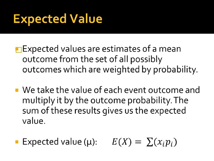
Expected Value �

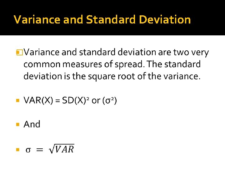
Variance and Standard Deviation �

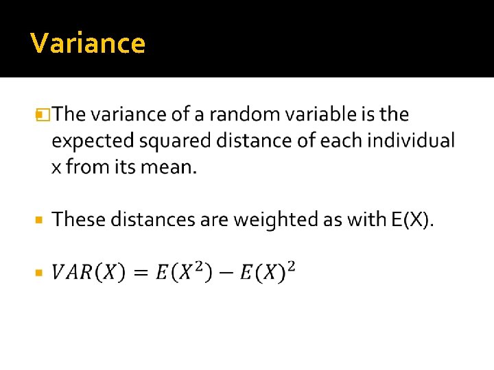
Variance �

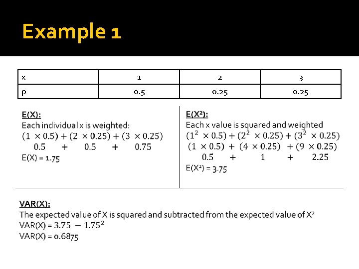
Example 1 x 1 2 3 p 0. 5 0. 25

Linear functions of a random variable �When given a linear function ‘y’ that acts upon a random variable ‘x’ we can also find expected values and variance of that function - E(Y) and VAR(Y). �From working through a simple example we can see how the function affects E(X) and VAR(X).

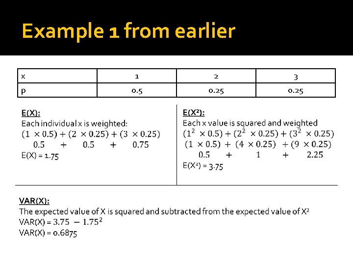
Example 1 from earlier x 1 2 3 p 0. 5 0. 25

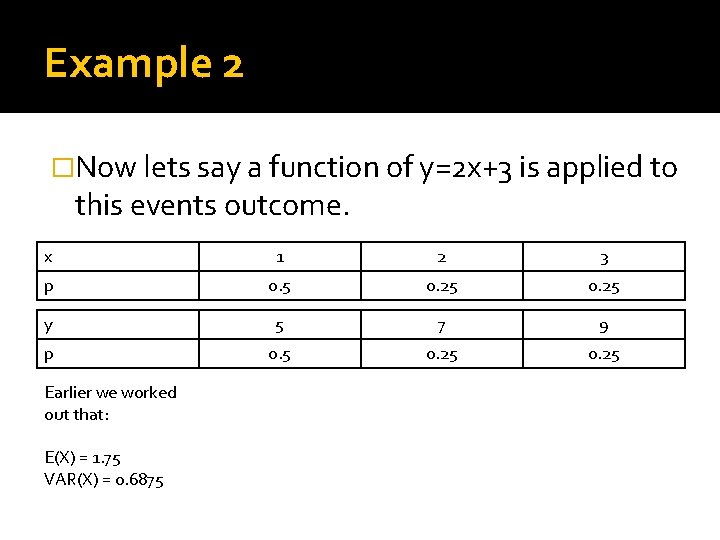
Example 2 �Now lets say a function of y=2 x+3 is applied to this events outcome. x 1 2 3 p 0. 5 0. 25 y 5 7 9 p 0. 5 0. 25 Earlier we worked out that: E(X) = 1. 75 VAR(X) = 0. 6875

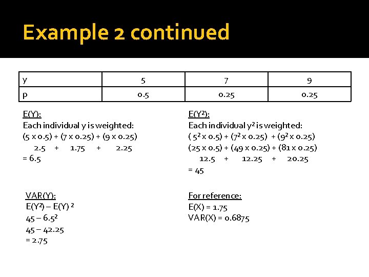
Example 2 continued y 5 7 9 p 0. 5 0. 25 E(Y): Each individual y is weighted: (5 x 0. 5) + (7 x 0. 25) + (9 x 0. 25) 2. 5 + 1. 75 + 2. 25 = 6. 5 VAR(Y): E(Y²) – E(Y) ² 45 – 6. 5² 45 – 42. 25 = 2. 75 E(Y²): Each individual y² is weighted: ( 5² x 0. 5) + (7² x 0. 25) + (9² x 0. 25) (25 x 0. 5) + (49 x 0. 25) + (81 x 0. 25) 12. 5 + 12. 25 + 20. 25 = 45 For reference: E(X) = 1. 75 VAR(X) = 0. 6875

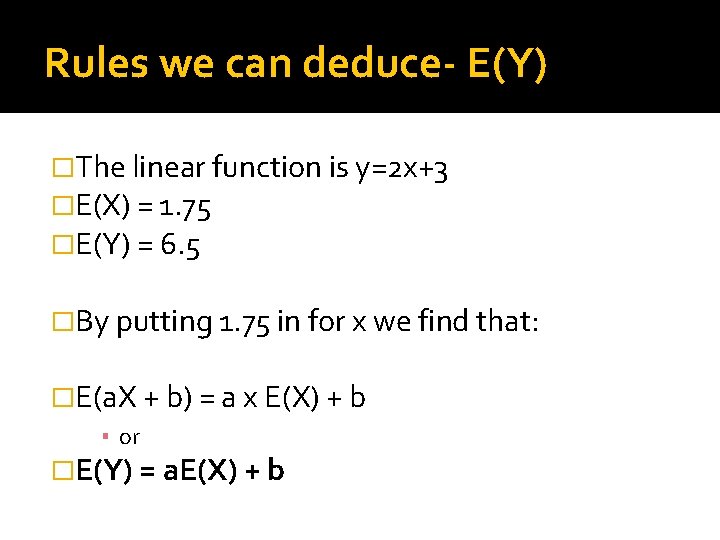
Rules we can deduce- E(Y) �The linear function is y=2 x+3 �E(X) = 1. 75 �E(Y) = 6. 5 �By putting 1. 75 in for x we find that: �E(a. X + b) = a x E(X) + b ▪ or �E(Y) = a. E(X) + b

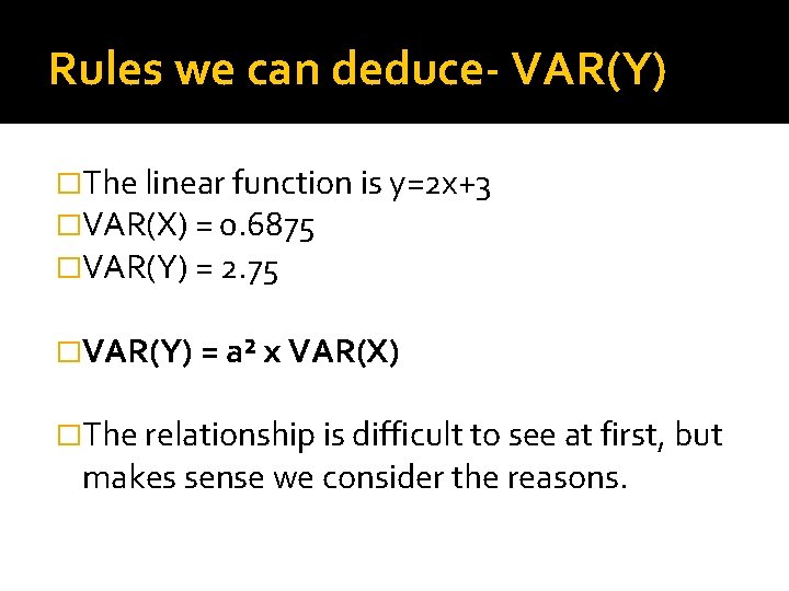
Rules we can deduce- VAR(Y) �The linear function is y=2 x+3 �VAR(X) = 0. 6875 �VAR(Y) = 2. 75 �VAR(Y) = a² x VAR(X) �The relationship is difficult to see at first, but makes sense we consider the reasons.

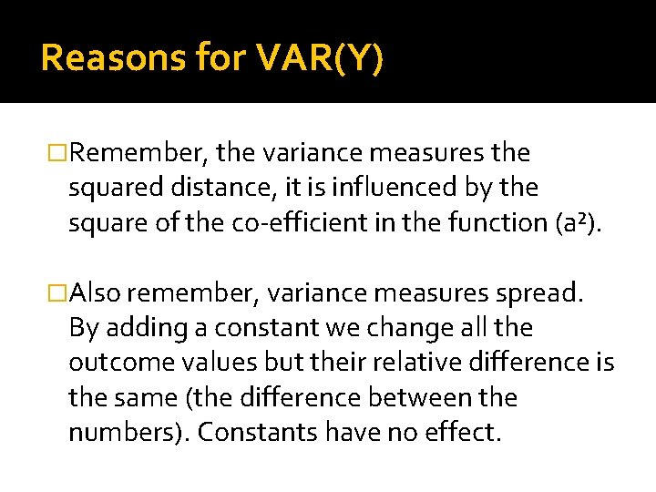
Reasons for VAR(Y) �Remember, the variance measures the squared distance, it is influenced by the square of the co-efficient in the function (a²). �Also remember, variance measures spread. By adding a constant we change all the outcome values but their relative difference is the same (the difference between the numbers). Constants have no effect.

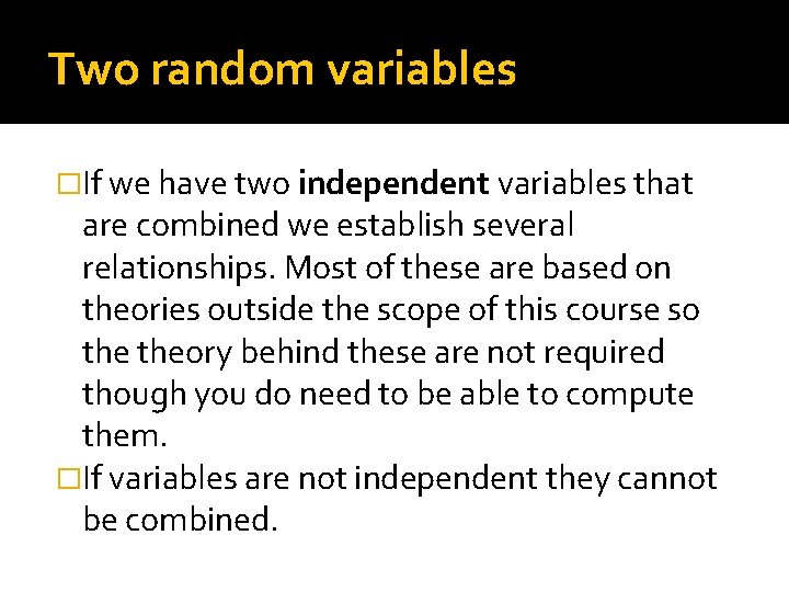
Two random variables �If we have two independent variables that are combined we establish several relationships. Most of these are based on theories outside the scope of this course so theory behind these are not required though you do need to be able to compute them. �If variables are not independent they cannot be combined.

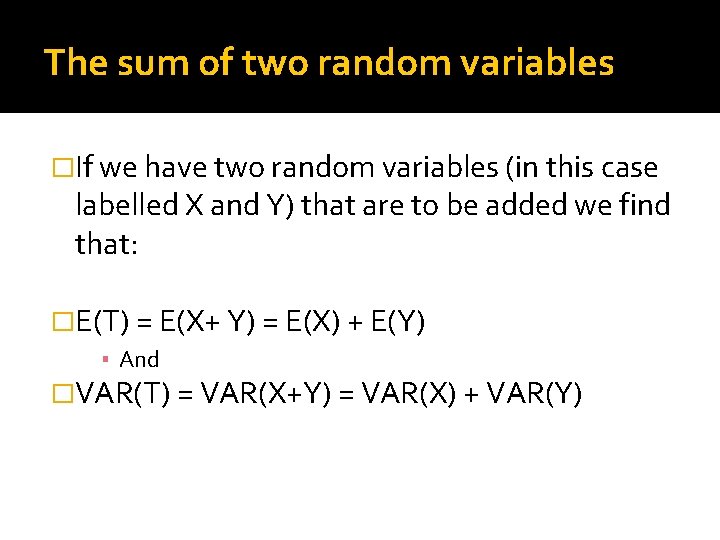
The sum of two random variables �If we have two random variables (in this case labelled X and Y) that are to be added we find that: �E(T) = E(X+ Y) = E(X) + E(Y) ▪ And �VAR(T) = VAR(X+Y) = VAR(X) + VAR(Y)

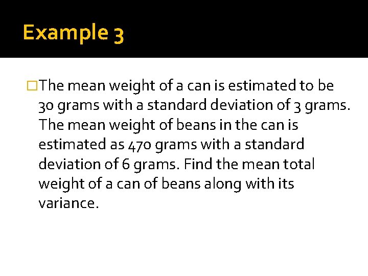
Example 3 �The mean weight of a can is estimated to be 30 grams with a standard deviation of 3 grams. The mean weight of beans in the can is estimated as 470 grams with a standard deviation of 6 grams. Find the mean total weight of a can of beans along with its variance.

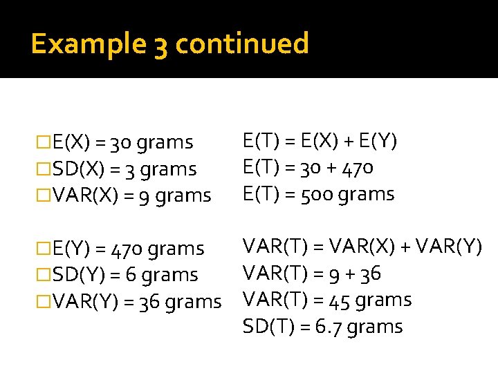
Example 3 continued �E(X) = 30 grams �SD(X) = 3 grams �VAR(X) = 9 grams E(T) = E(X) + E(Y) E(T) = 30 + 470 E(T) = 500 grams �E(Y) = 470 grams �SD(Y) = 6 grams �VAR(Y) = 36 grams VAR(T) = VAR(X) + VAR(Y) VAR(T) = 9 + 36 VAR(T) = 45 grams SD(T) = 6. 7 grams

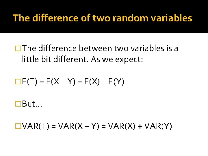
The difference of two random variables �The difference between two variables is a little bit different. As we expect: �E(T) = E(X – Y) = E(X) – E(Y) �But… �VAR(T) = VAR(X – Y) = VAR(X) + VAR(Y)

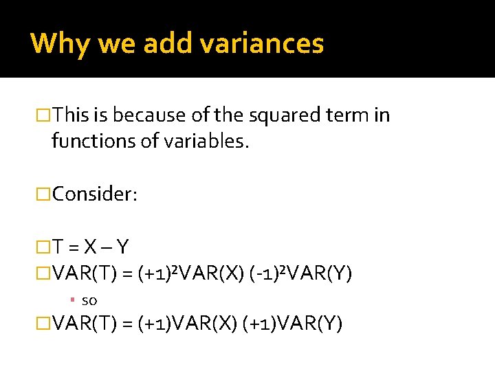
Why we add variances �This is because of the squared term in functions of variables. �Consider: �T = X – Y �VAR(T) = (+1)²VAR(X) (-1)²VAR(Y) ▪ so �VAR(T) = (+1)VAR(X) (+1)VAR(Y)

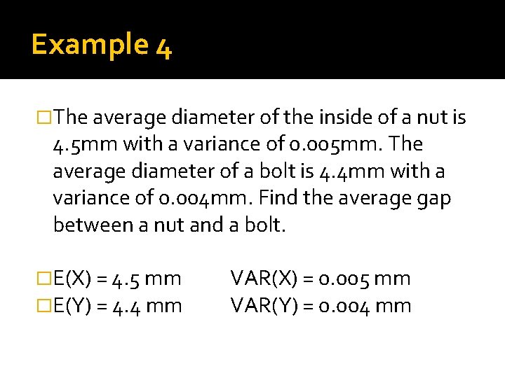
Example 4 �The average diameter of the inside of a nut is 4. 5 mm with a variance of 0. 005 mm. The average diameter of a bolt is 4. 4 mm with a variance of 0. 004 mm. Find the average gap between a nut and a bolt. �E(X) = 4. 5 mm �E(Y) = 4. 4 mm VAR(X) = 0. 005 mm VAR(Y) = 0. 004 mm

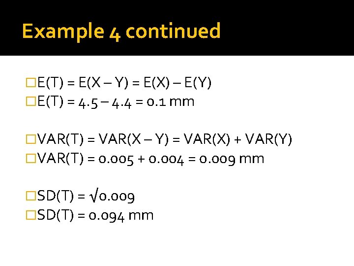
Example 4 continued �E(T) = E(X – Y) = E(X) – E(Y) �E(T) = 4. 5 – 4. 4 = 0. 1 mm �VAR(T) = VAR(X – Y) = VAR(X) + VAR(Y) �VAR(T) = 0. 005 + 0. 004 = 0. 009 mm �SD(T) = √ 0. 009 �SD(T) = 0. 094 mm

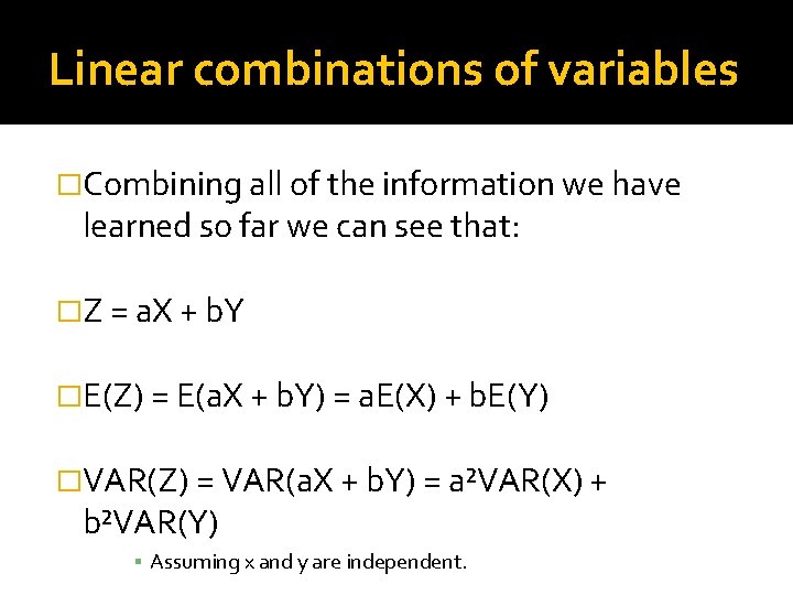
Linear combinations of variables �Combining all of the information we have learned so far we can see that: �Z = a. X + b. Y �E(Z) = E(a. X + b. Y) = a. E(X) + b. E(Y) �VAR(Z) = VAR(a. X + b. Y) = a²VAR(X) + b²VAR(Y) ▪ Assuming x and y are independent.

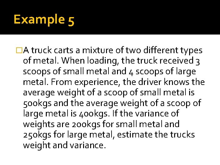
Example 5 �A truck carts a mixture of two different types of metal. When loading, the truck received 3 scoops of small metal and 4 scoops of large metal. From experience, the driver knows the average weight of a scoop of small metal is 500 kgs and the average weight of a scoop of large metal is 400 kgs. If the variance of weights are 200 kgs for small metal and 250 kgs for large metal, estimate the trucks weight and variance.

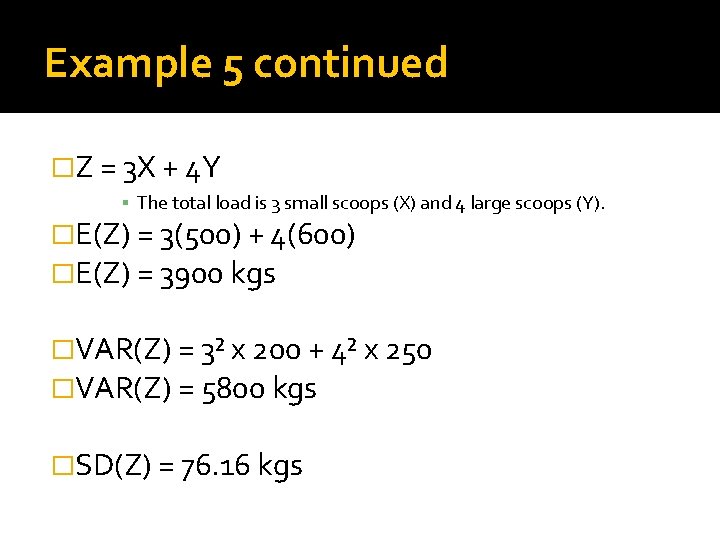
Example 5 continued �Z = 3 X + 4 Y ▪ The total load is 3 small scoops (X) and 4 large scoops (Y). �E(Z) = 3(500) + 4(600) �E(Z) = 3900 kgs �VAR(Z) = 3² x 200 + 4² x 250 �VAR(Z) = 5800 kgs �SD(Z) = 76. 16 kgs