Expectation Let X denote a discrete random variable

Expectation

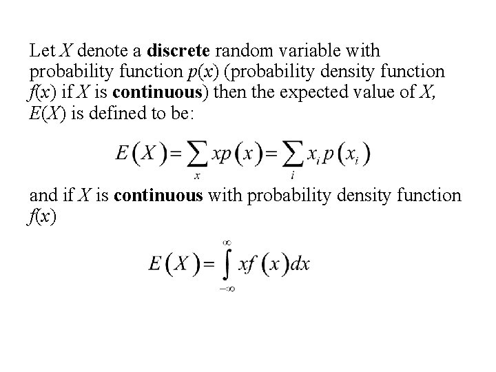
Let X denote a discrete random variable with probability function p(x) (probability density function f(x) if X is continuous) then the expected value of X, E(X) is defined to be: and if X is continuous with probability density function f(x)

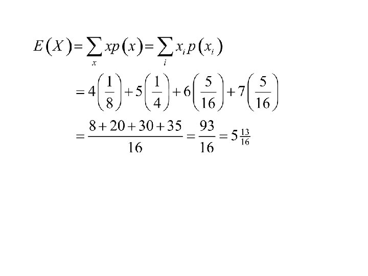
Example: Suppose we are observing a seven game series where the teams are evenly matched and the games are independent. Let X denote the length of the series. Find: 1. The distribution of X. 2. the expected value of X, E(X).

Solution: Let A denote the event that team A, wins and B denote the event that team B wins. Then the sample space for this experiment (together with probabilities and values of X) would be (next slide):

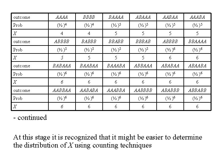
outcome AAAA BBBB BAAAA ABAAA AABAA AAABA Prob (½ )4 (½ )5 4 4 5 5 ABBBB BABBB BBABB BBBAB ABBBB BBAAAA (½ )5 (½ )6 5 5 6 6 BABAAA BAABAA BAAABA ABBAAA ABABAABA (½ )6 (½ )6 6 6 6 AABBAA AABABA AAABBA AABBBB ABABBB ABBABB (½ )6 (½ )6 6 6 6 X outcome Prob X - continued At this stage it is recognized that it might be easier to determine the distribution of X using counting techniques

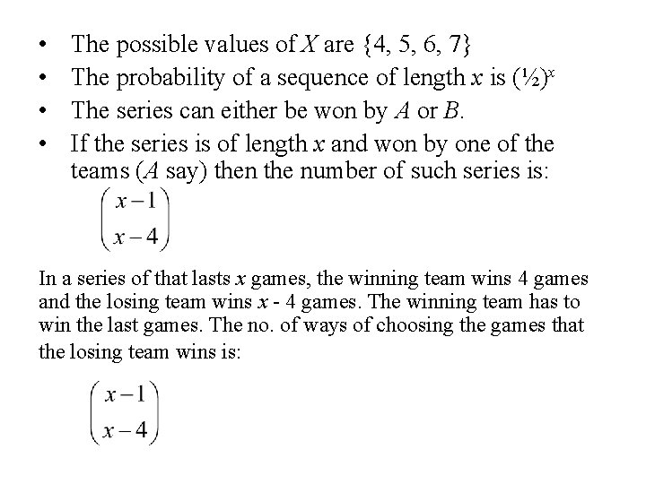
• • The possible values of X are {4, 5, 6, 7} The probability of a sequence of length x is (½)x The series can either be won by A or B. If the series is of length x and won by one of the teams (A say) then the number of such series is: In a series of that lasts x games, the winning team wins 4 games and the losing team wins x - 4 games. The winning team has to win the last games. The no. of ways of choosing the games that the losing team wins is:

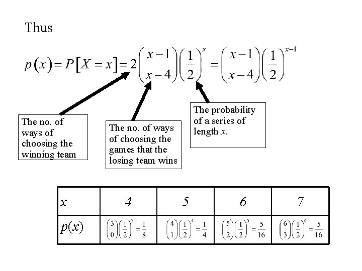
Thus The no. of ways of choosing the winning team x p(x) The probability of a series of length x. The no. of ways of choosing the games that the losing team wins 4 5 6 7

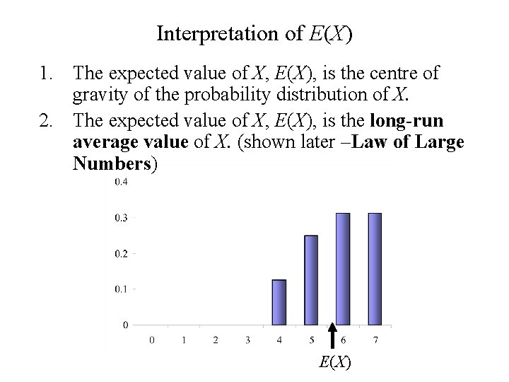
Interpretation of E(X) 1. The expected value of X, E(X), is the centre of gravity of the probability distribution of X. 2. The expected value of X, E(X), is the long-run average value of X. (shown later –Law of Large Numbers) E(X)

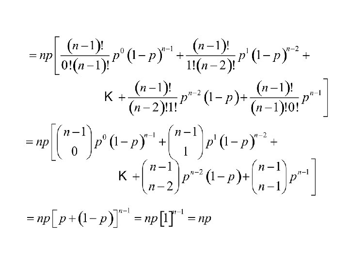
Example: The Binomal distribution Let X be a discrete random variable having the Binomial distribution. i. e. X = the number of successes in n independent repetitions of a Bernoulli trial. Find the expected value of X, E(X).

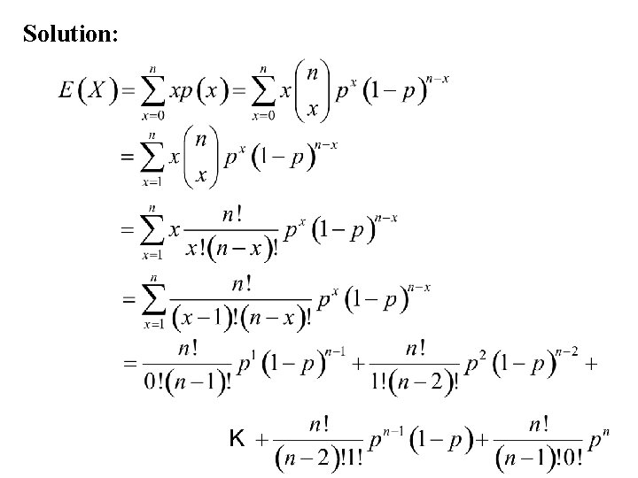
Solution:

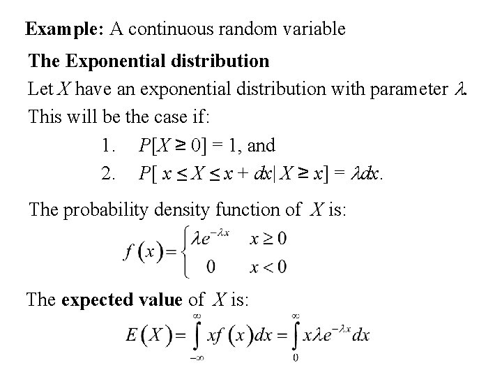
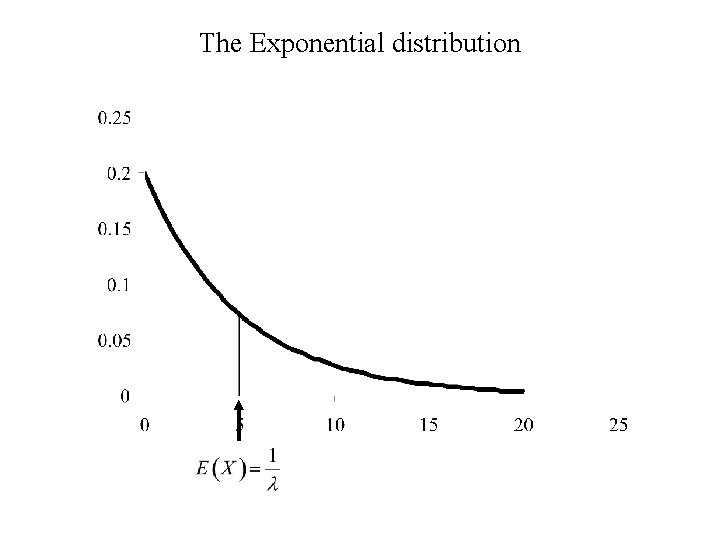
Example: A continuous random variable The Exponential distribution Let X have an exponential distribution with parameter l. This will be the case if: 1. P[X ≥ 0] = 1, and 2. P[ x ≤ X ≤ x + dx| X ≥ x] = ldx. The probability density function of X is: The expected value of X is:

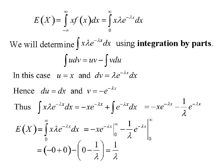
We will determine using integration by parts.

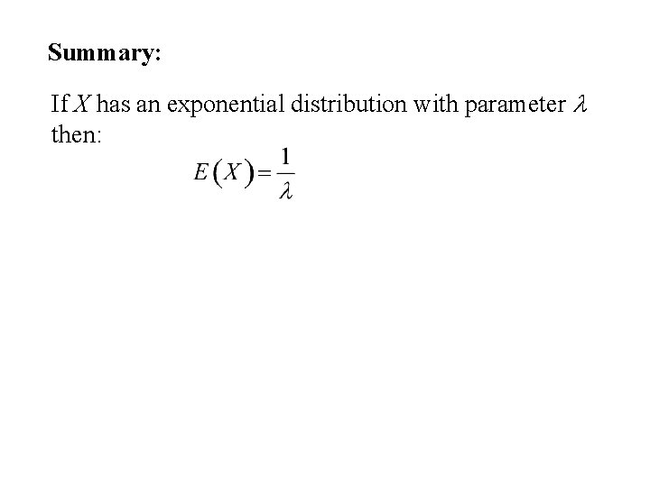
Summary: If X has an exponential distribution with parameter l then:

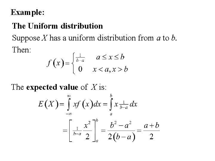
Example: The Uniform distribution Suppose X has a uniform distribution from a to b. Then: The expected value of X is:

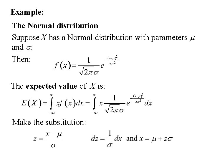
Example: The Normal distribution Suppose X has a Normal distribution with parameters m and s. Then: The expected value of X is: Make the substitution:

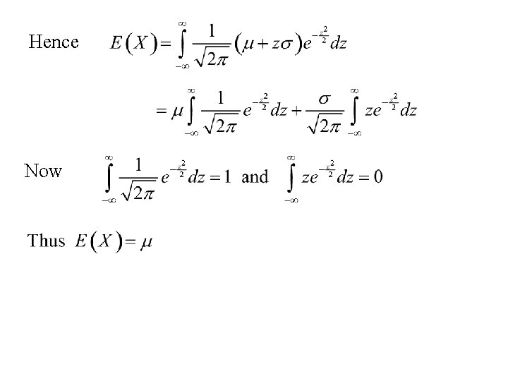
Hence Now

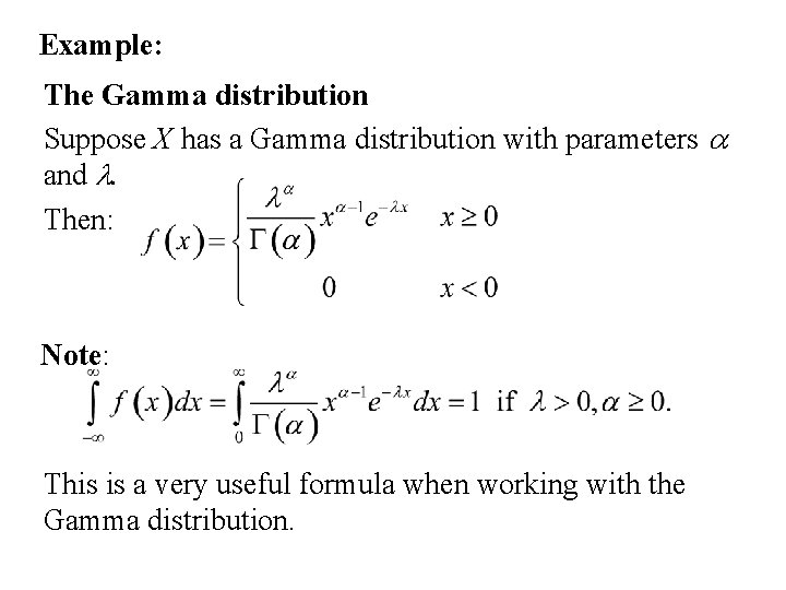
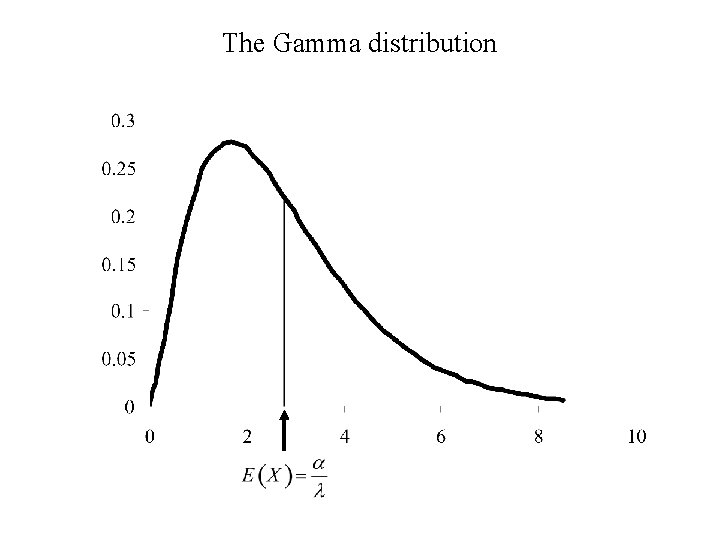
Example: The Gamma distribution Suppose X has a Gamma distribution with parameters a and l. Then: Note: This is a very useful formula when working with the Gamma distribution.

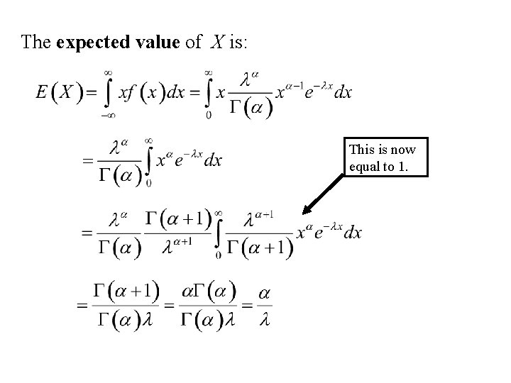
The expected value of X is: This is now equal to 1.

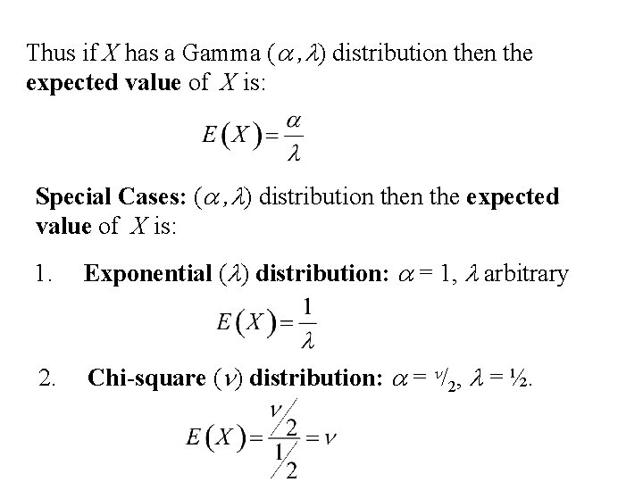
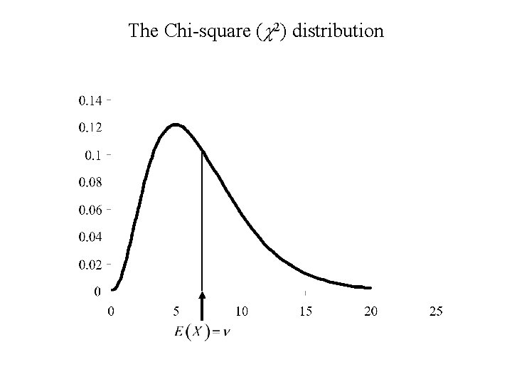
Thus if X has a Gamma (a , l) distribution the expected value of X is: Special Cases: (a , l) distribution the expected value of X is: 1. Exponential (l) distribution: a = 1, l arbitrary 2. Chi-square (n) distribution: a = n/2, l = ½.

The Gamma distribution

The Exponential distribution

The Chi-square (c 2) distribution

Expectation of functions of Random Variables

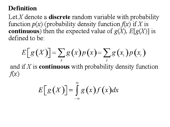
Definition Let X denote a discrete random variable with probability function p(x) (probability density function f(x) if X is continuous) then the expected value of g(X), E[g(X)] is defined to be: and if X is continuous with probability density function f(x)

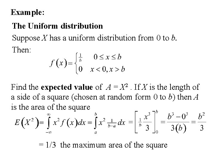
Example: The Uniform distribution Suppose X has a uniform distribution from 0 to b. Then: Find the expected value of A = X 2. If X is the length of a side of a square (chosen at random form 0 to b) then A is the area of the square = 1/3 the maximum area of the square

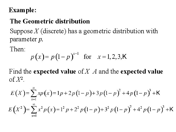
Example: The Geometric distribution Suppose X (discrete) has a geometric distribution with parameter p. Then: Find the expected value of X A and the expected value of X 2.

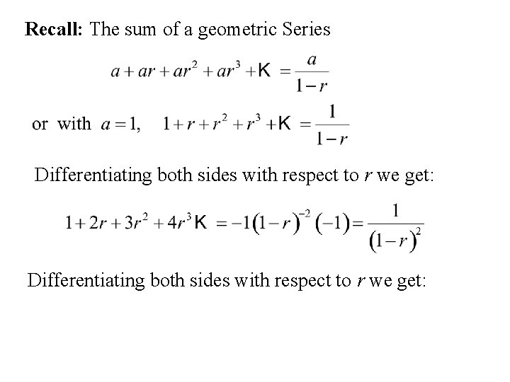
Recall: The sum of a geometric Series Differentiating both sides with respect to r we get:

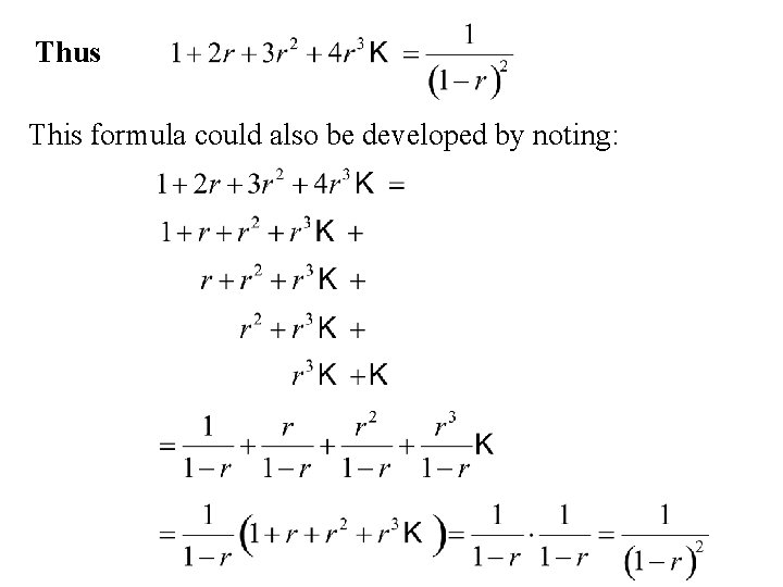
Thus This formula could also be developed by noting:

This formula can be used to calculate:

To compute the expected value of X 2. we need to find a formula for Note Differentiating with respect to r we get

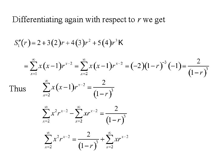
Differentiating again with respect to r we get Thus

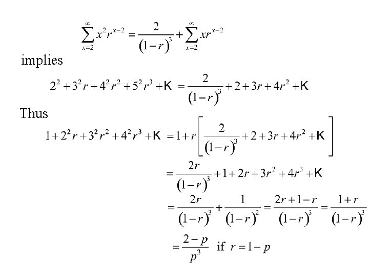
implies Thus

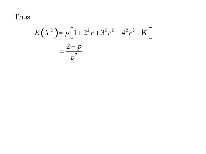
Thus

Moments of Random Variables

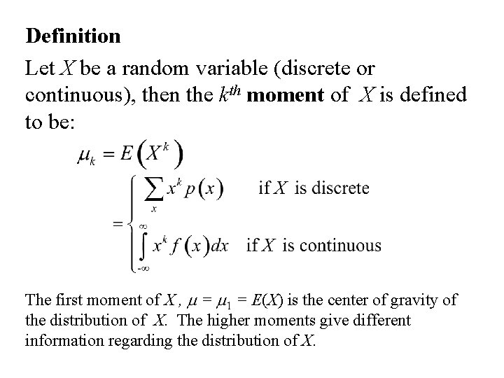
Definition Let X be a random variable (discrete or continuous), then the kth moment of X is defined to be: The first moment of X , m = m 1 = E(X) is the center of gravity of the distribution of X. The higher moments give different information regarding the distribution of X.

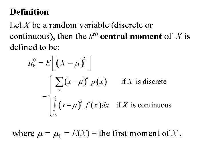
Definition Let X be a random variable (discrete or continuous), then the kth central moment of X is defined to be: where m = m 1 = E(X) = the first moment of X.

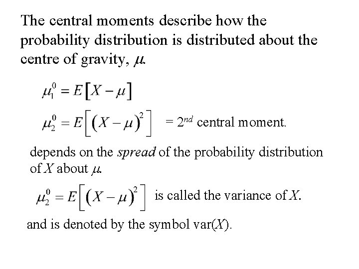
The central moments describe how the probability distribution is distributed about the centre of gravity, m. = 2 nd central moment. depends on the spread of the probability distribution of X about m. is called the variance of X. and is denoted by the symbol var(X).

is called the standard deviation of X and is denoted by the symbol s. The third central moment contains information about the skewness of a distribution.

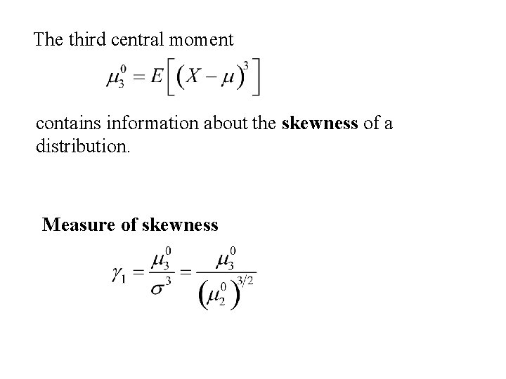
The third central moment contains information about the skewness of a distribution. Measure of skewness

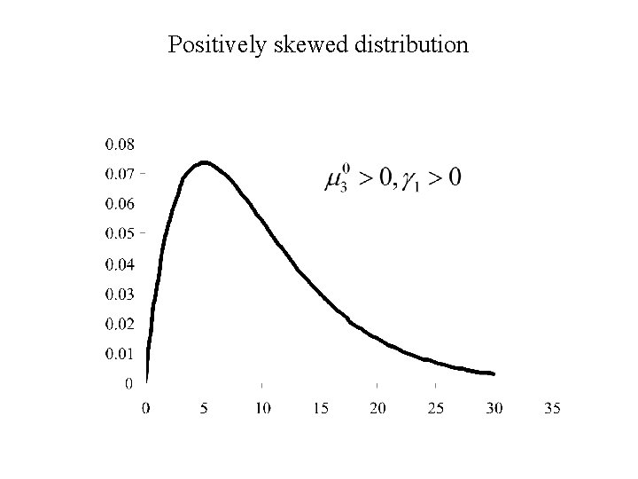
Positively skewed distribution

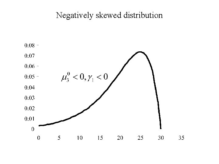
Negatively skewed distribution

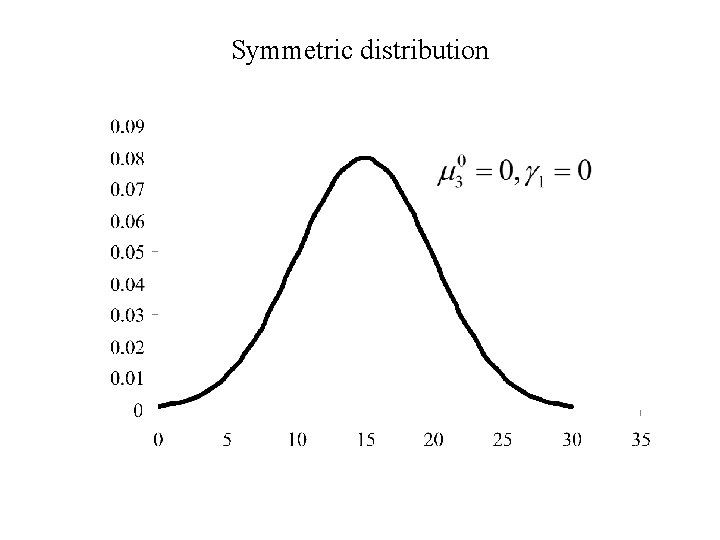
Symmetric distribution

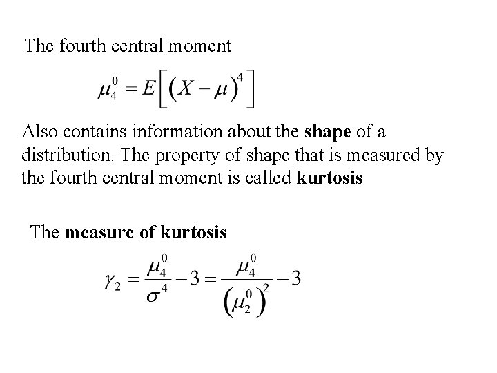
The fourth central moment Also contains information about the shape of a distribution. The property of shape that is measured by the fourth central moment is called kurtosis The measure of kurtosis

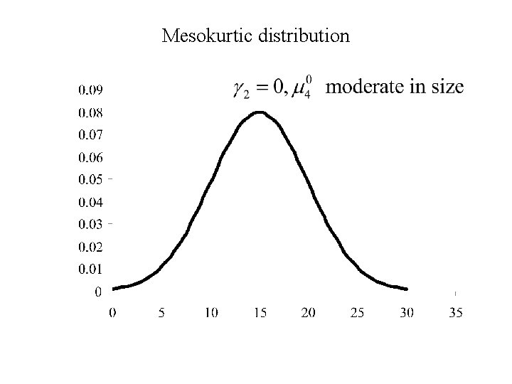
Mesokurtic distribution

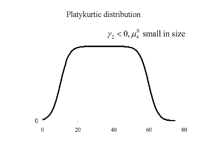
Platykurtic distribution

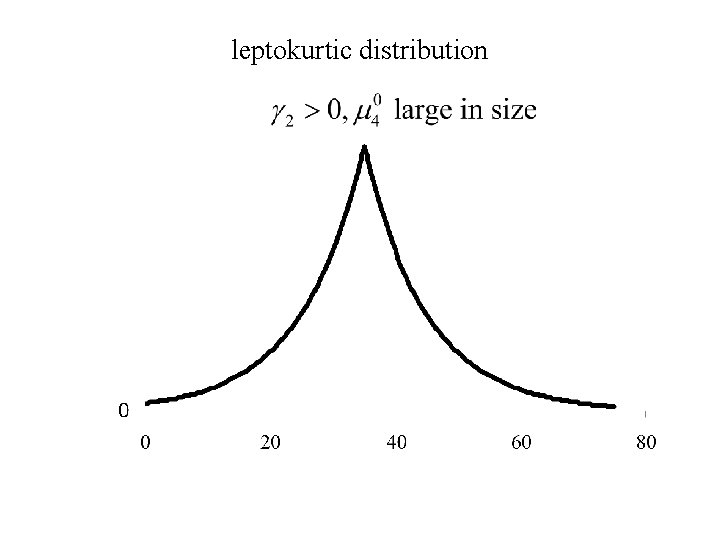
leptokurtic distribution

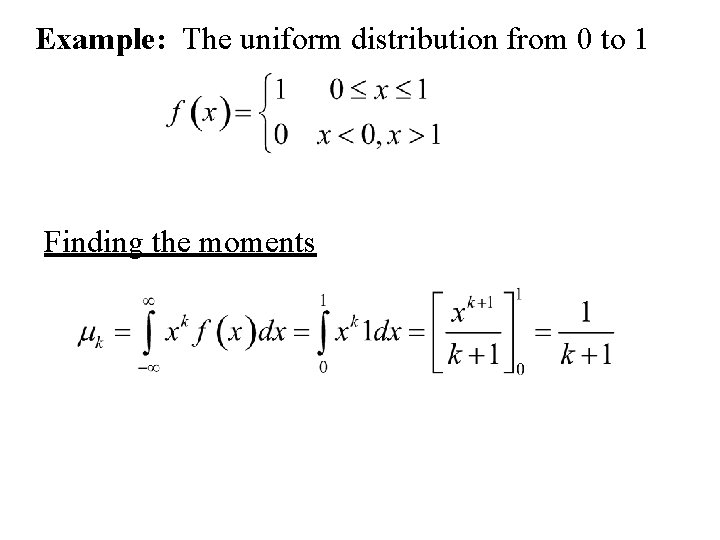
Example: The uniform distribution from 0 to 1 Finding the moments

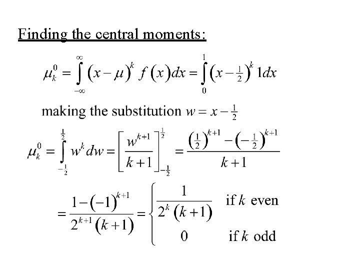
Finding the central moments:

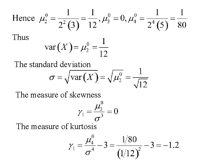
Thus The standard deviation The measure of skewness The measure of kurtosis

Rules for expectation

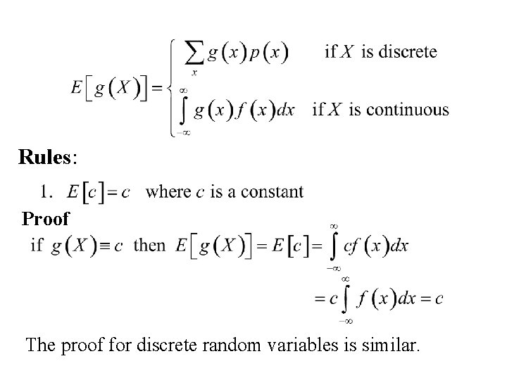
Rules: Proof The proof for discrete random variables is similar.

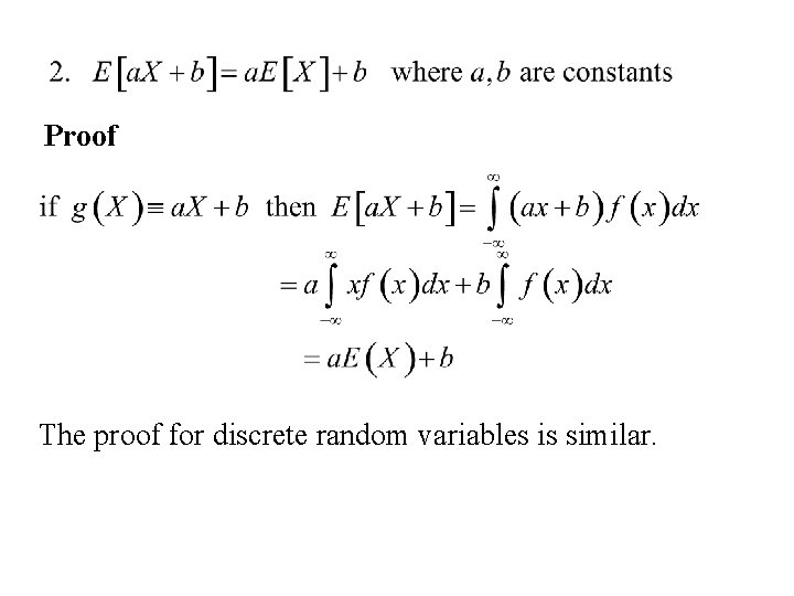
Proof The proof for discrete random variables is similar.

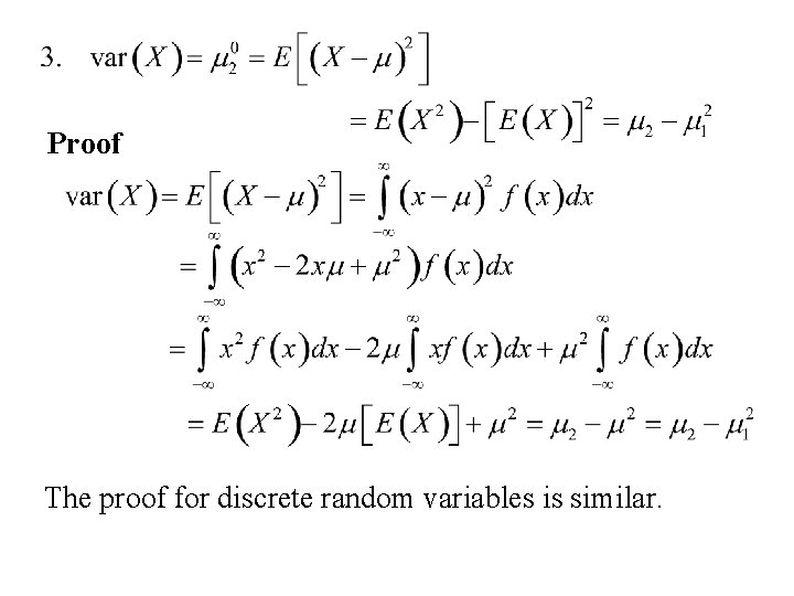
Proof The proof for discrete random variables is similar.

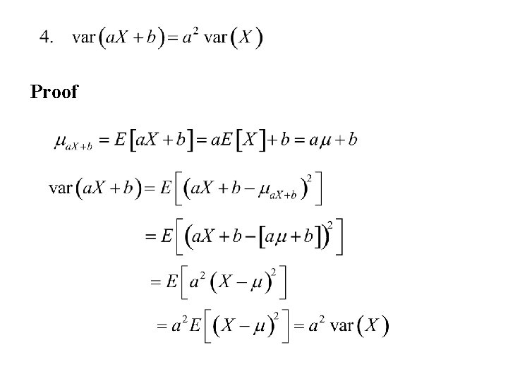
Proof

Moment generating functions

Recall Definition Let X denote a random variable, Then the moment generating function of X , m. X(t) is defined by:

Examples 1. The Binomial distribution (parameters p, n) The moment generating function of X , m. X(t) is:

2. The Poisson distribution (parameter l) The moment generating function of X , m. X(t) is:

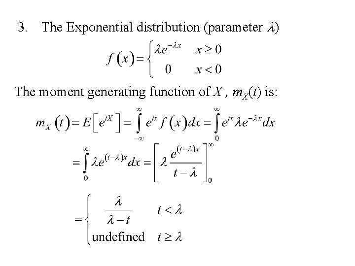
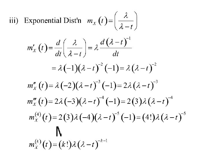
3. The Exponential distribution (parameter l) The moment generating function of X , m. X(t) is:

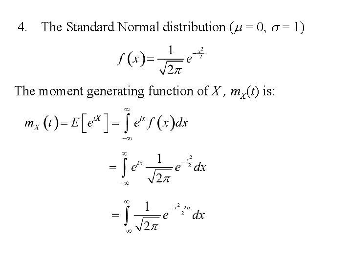
4. The Standard Normal distribution (m = 0, s = 1) The moment generating function of X , m. X(t) is:

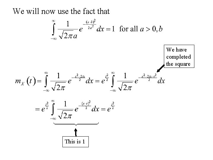
We will now use the fact that We have completed the square This is 1

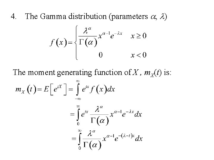
4. The Gamma distribution (parameters a, l) The moment generating function of X , m. X(t) is:

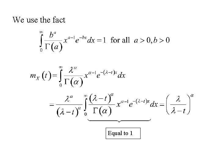
We use the fact Equal to 1

Properties of Moment Generating Functions

1. m. X(0) = 1 Note: the moment generating functions of the following distributions satisfy the property m. X(0) = 1

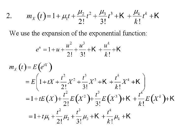
We use the expansion of the exponential function:

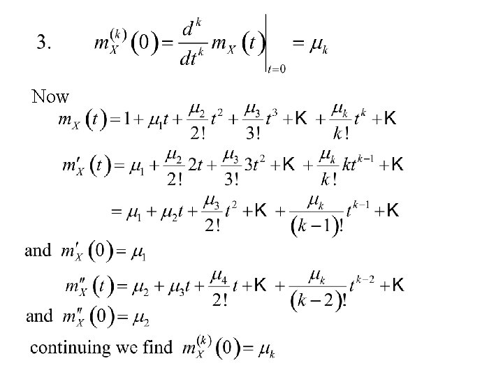
Now

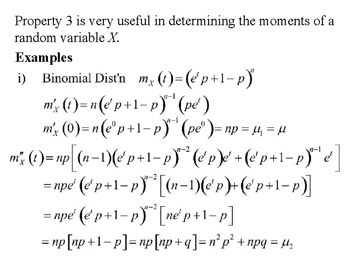
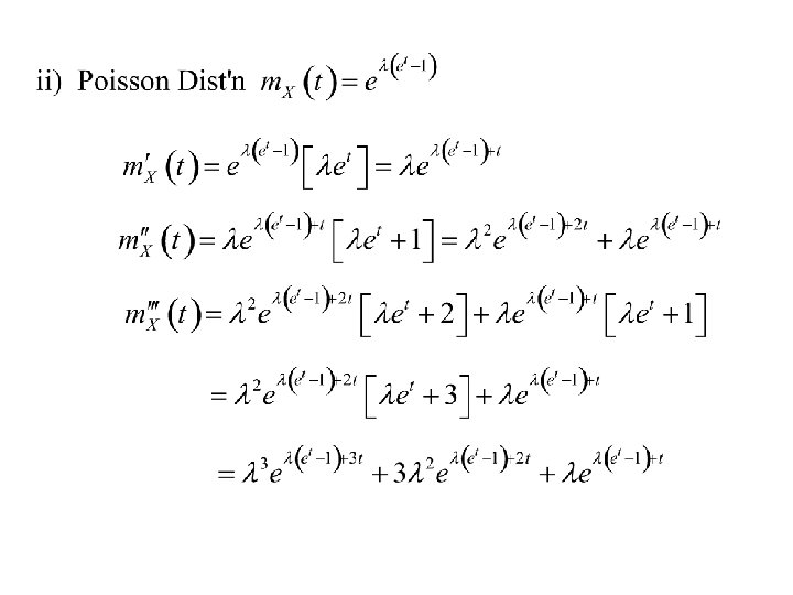
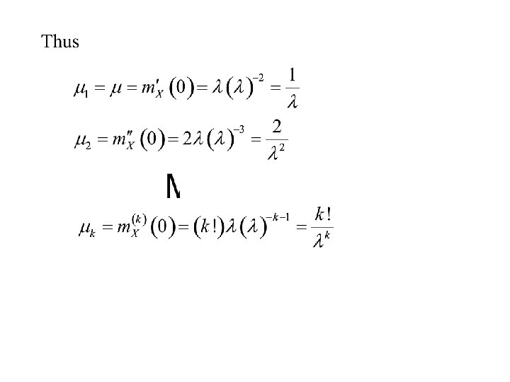
Property 3 is very useful in determining the moments of a random variable X. Examples

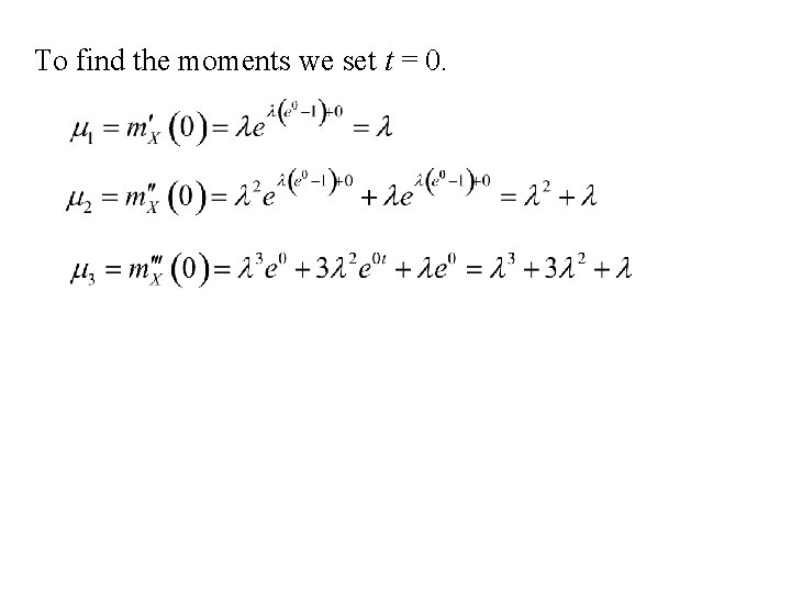
To find the moments we set t = 0.

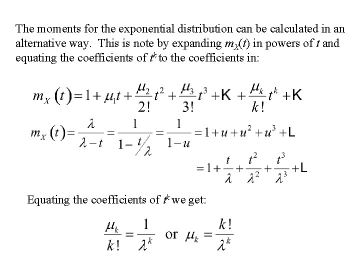
The moments for the exponential distribution can be calculated in an alternative way. This is note by expanding m. X(t) in powers of t and equating the coefficients of tk to the coefficients in: Equating the coefficients of tk we get:

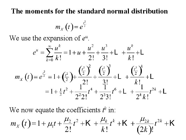
The moments for the standard normal distribution We use the expansion of eu. We now equate the coefficients tk in:

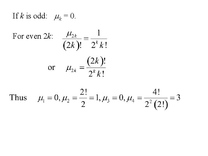
If k is odd: mk = 0. For even 2 k: