Expanders Eliyahu Kiperwasser What is it l Expanders

Expanders Eliyahu Kiperwasser

What is it? l Expanders are graphs with no small cuts. The later gives several unique traits to such graph, such as: – – High connectivity. No “bottle-neck”.

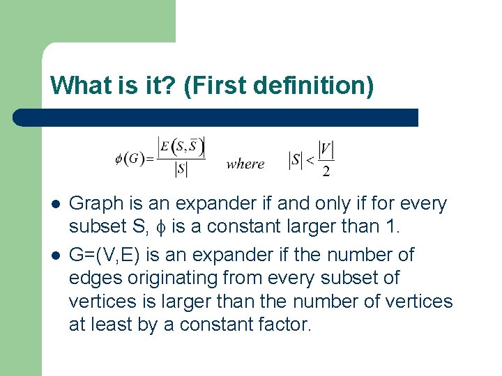
What is it? (First definition) l l Graph is an expander if and only if for every subset S, is a constant larger than 1. G=(V, E) is an expander if the number of edges originating from every subset of vertices is larger than the number of vertices at least by a constant factor.

That’s Easy… l We are all familiar with graphs which are in fact expanders with more than a constant factor. – l i. e. cliques. The challenge is to find sparse graphs which hold as expanders.

Construction of Explicit Expanders l l In this section, we describe two ways to build such marvelous objects as expanders. The following two methods show that some constant-degree regular graph exist with good expansion. We will show: – – The Margulis/Gaber-Galil Expander. The Lubotsky-Philips-Sarnak Expander.

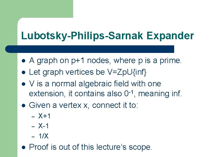
Lubotsky-Philips-Sarnak Expander l l A graph on p+1 nodes, where p is a prime. Let graph vertices be V=Zp. U{inf} V is a normal algebraic field with one extension, it contains also 0 -1, meaning inf. Given a vertex x, connect it to: – – – l X+1 X-1 1/X Proof is out of this lecture’s scope.

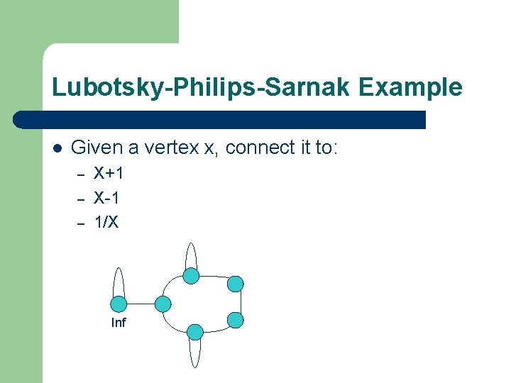
Lubotsky-Philips-Sarnak Example l Given a vertex x, connect it to: – – – X+1 X-1 1/X Inf

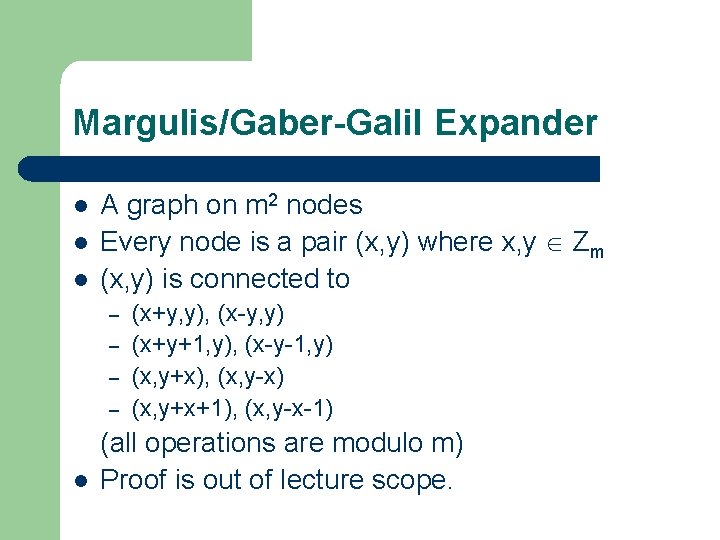
Margulis/Gaber-Galil Expander l l l A graph on m 2 nodes Every node is a pair (x, y) where x, y Zm (x, y) is connected to – – l (x+y, y), (x-y, y) (x+y+1, y), (x-y-1, y) (x, y+x), (x, y-x) (x, y+x+1), (x, y-x-1) (all operations are modulo m) Proof is out of lecture scope.

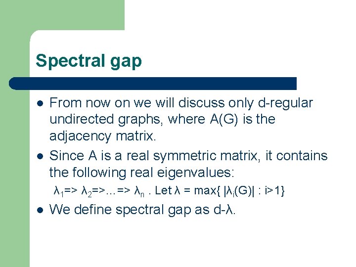
Spectral gap l l From now on we will discuss only d-regular undirected graphs, where A(G) is the adjacency matrix. Since A is a real symmetric matrix, it contains the following real eigenvalues: λ 1=> λ 2=>…=> λn. Let λ = max{ |λi(G)| : i>1} l We define spectral gap as d-λ.

A second definition of expanders l l We can define an expander graph by looking at the adjacency matrix A. Graph is an expander if and only if A’s spectral gap is larger than zero.

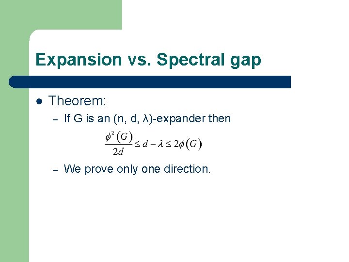
Expansion vs. Spectral gap l Theorem: – If G is an (n, d, λ)-expander then – We prove only one direction.

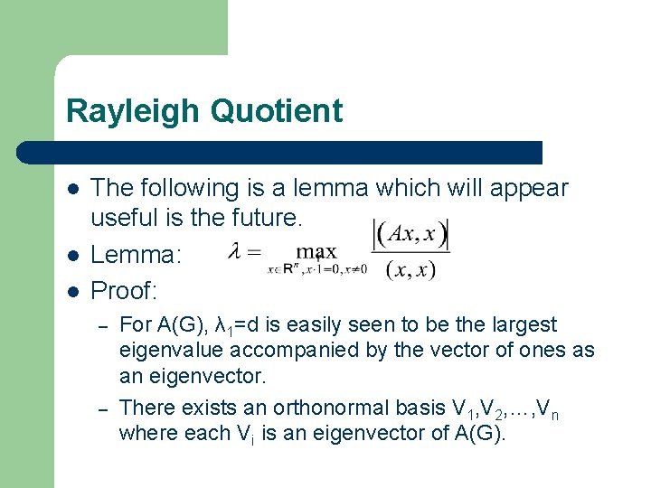
Rayleigh Quotient l l l The following is a lemma which will appear useful is the future. Lemma: Proof: – – For A(G), λ 1=d is easily seen to be the largest eigenvalue accompanied by the vector of ones as an eigenvector. There exists an orthonormal basis V 1, V 2, …, Vn where each Vi is an eigenvector of A(G).

Rayleigh Quotient l Proof cont.

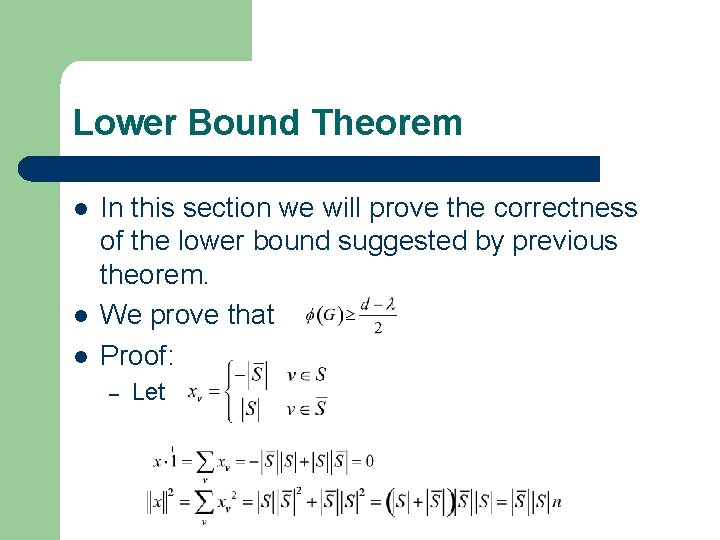
Lower Bound Theorem l l l In this section we will prove the correctness of the lower bound suggested by previous theorem. We prove that Proof: – Let

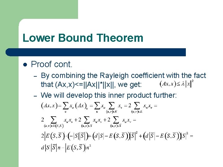
Lower Bound Theorem l Proof cont. – – By combining the Rayleigh coefficient with the fact that (Ax, x)<=||Ax||*||x||, we get: We will develop this inner product further:

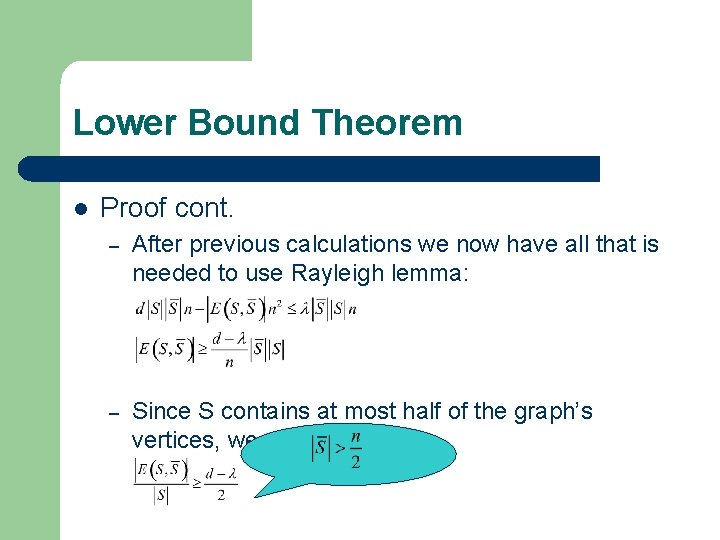
Lower Bound Theorem l Proof cont. – After previous calculations we now have all that is needed to use Rayleigh lemma: – Since S contains at most half of the graph’s vertices, we conclude:

Markov Chains l l l Definition: A finite state machine with probabilities for each transition, that is, a probability that the next state is j given that the current state is i. Named after Andrei Andreyevich Markov (1856 - 1922), who studied poetry and other texts as stochastic sequences of characters. We will use Markov chains for the proof of our next final lemma, in order to analyze a random walk on an expander graph.

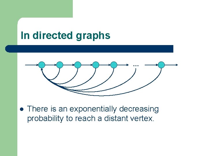
In directed graphs … l There is an exponentially decreasing probability to reach a distant vertex.

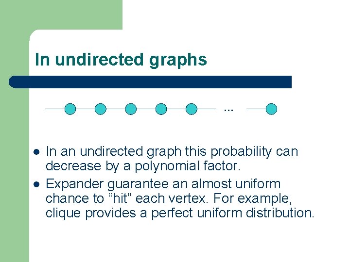
In undirected graphs … l l In an undirected graph this probability can decrease by a polynomial factor. Expander guarantee an almost uniform chance to “hit” each vertex. For example, clique provides a perfect uniform distribution.

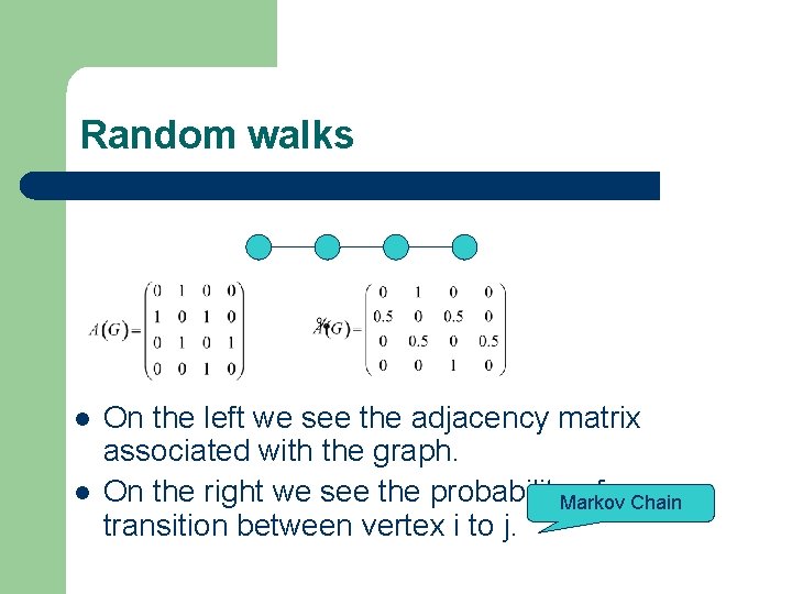
Random walks l l On the left we see the adjacency matrix associated with the graph. On the right we see the probability. Markov of Chain transition between vertex i to j.

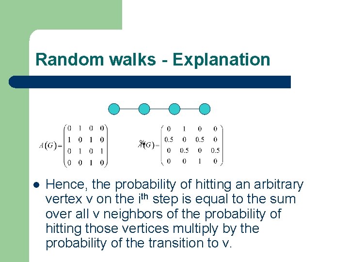
Random walks - Explanation l Hence, the probability of hitting an arbitrary vertex v on the ith step is equal to the sum over all v neighbors of the probability of hitting those vertices multiply by the probability of the transition to v.

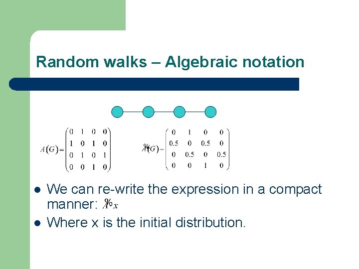
Random walks – Algebraic notation l l We can re-write the expression in a compact manner: Where x is the initial distribution.

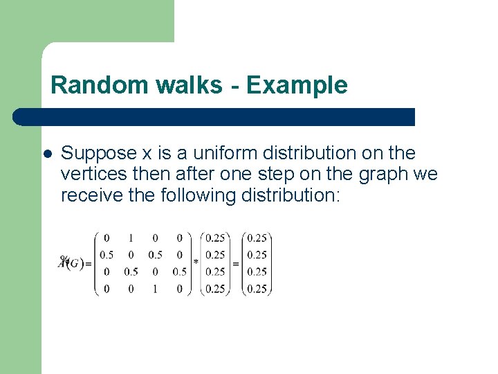
Random walks - Example l Suppose x is a uniform distribution on the vertices then after one step on the graph we receive the following distribution:

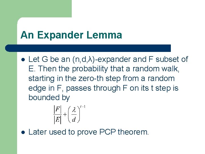
An Expander Lemma l Let G be an (n, d, λ)-expander and F subset of E. Then the probability that a random walk, starting in the zero-th step from a random edge in F, passes through F on its t step is bounded by l Later used to prove PCP theorem.

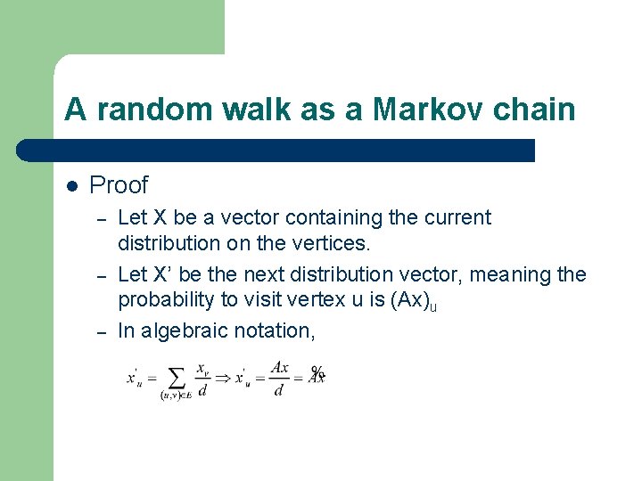
A random walk as a Markov chain l Proof – – – Let X be a vector containing the current distribution on the vertices. Let X’ be the next distribution vector, meaning the probability to visit vertex u is (Ax)u In algebraic notation,

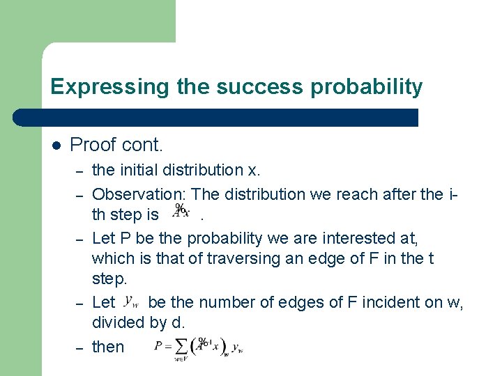
Expressing the success probability l Proof cont. – – – the initial distribution x. Observation: The distribution we reach after the ith step is. Let P be the probability we are interested at, which is that of traversing an edge of F in the t step. Let be the number of edges of F incident on w, divided by d. then

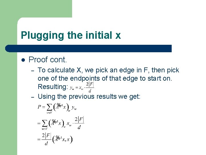
Plugging the initial x l Proof cont. – – To calculate X, we pick an edge in F, then pick one of the endpoints of that edge to start on. Resulting: Using the previous results we get:

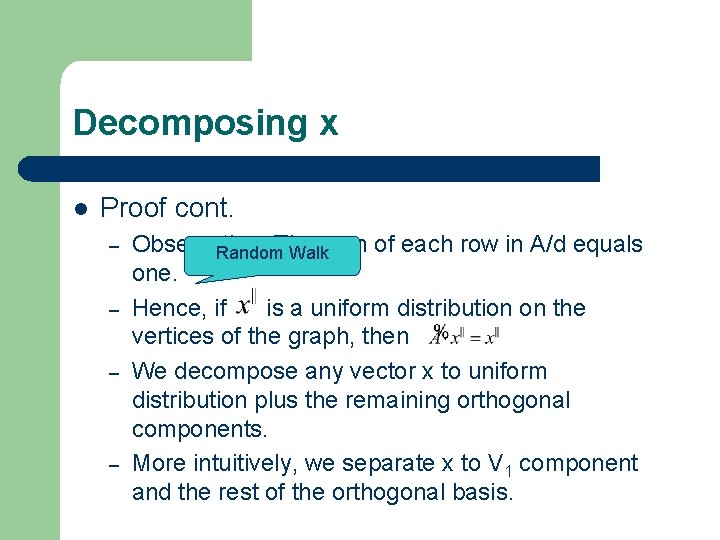
Decomposing x l Proof cont. – – Observation: The Random Walksum of each row in A/d equals one. Hence, if is a uniform distribution on the vertices of the graph, then We decompose any vector x to uniform distribution plus the remaining orthogonal components. More intuitively, we separate x to V 1 component and the rest of the orthogonal basis.

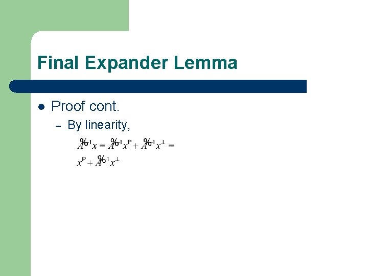
Final Expander Lemma l Proof cont. – By linearity,

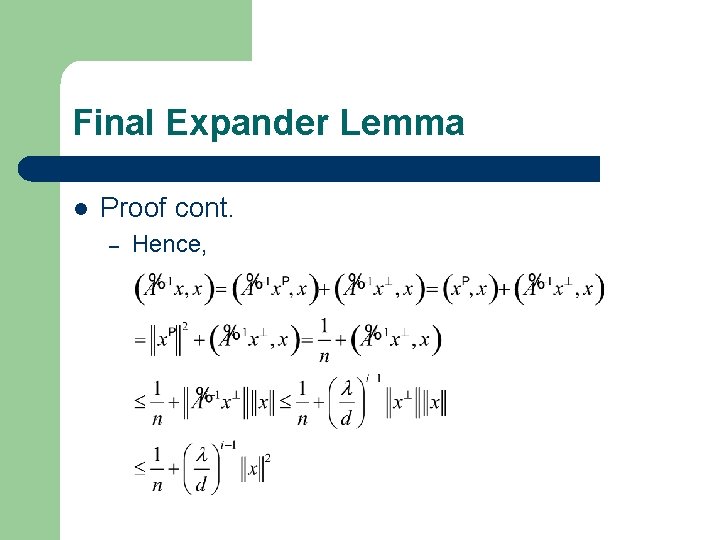
Final Expander Lemma l Proof cont. – Hence,

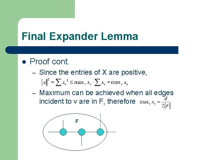
Final Expander Lemma l Proof cont. – Since the entries of X are positive, – Maximum can be achieved when all edges incident to v are in F, therefore F

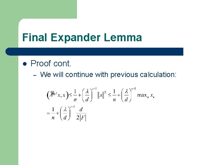
Final Expander Lemma l Proof cont. – We will continue with previous calculation:

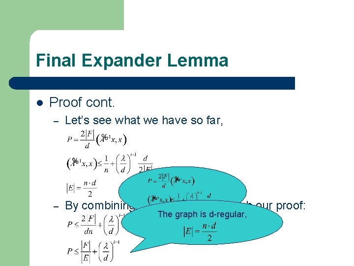
Final Expander Lemma l Proof cont. – Let’s see what we have so far, – By combining those result, we finish our proof: The graph is d-regular,

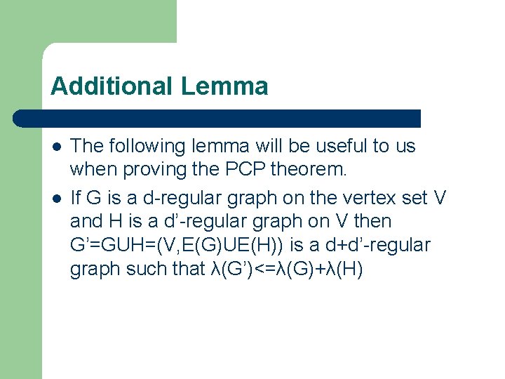
Additional Lemma l l The following lemma will be useful to us when proving the PCP theorem. If G is a d-regular graph on the vertex set V and H is a d’-regular graph on V then G’=GUH=(V, E(G)UE(H)) is a d+d’-regular graph such that λ(G’)<=λ(G)+λ(H)

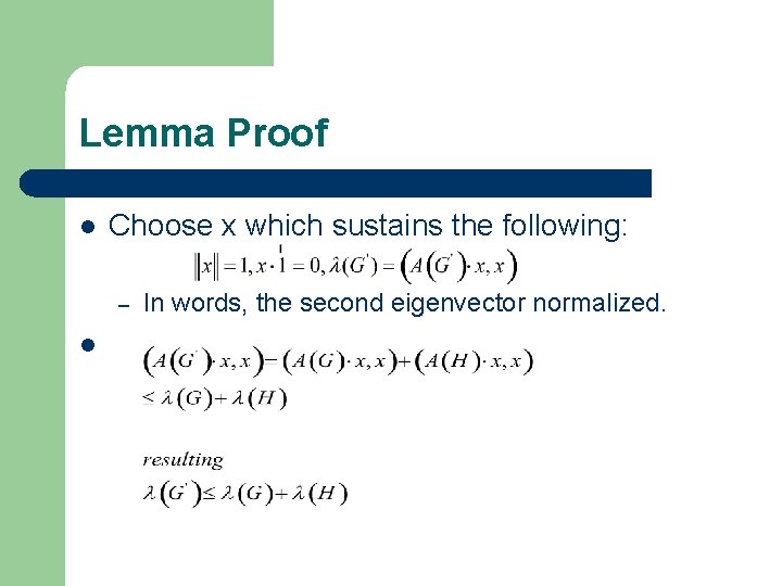
Lemma Proof l Choose x which sustains the following: – l In words, the second eigenvector normalized.

The End Questions?