Exercise 1 Entering data into SPSS 1 Open

Exercise 1: Entering data into SPSS 1. Open SPSS and select ‘New Dataset’ from the options 2. Go to ‘Variable View’ and create the dataset template for inputting the 5 variables on the handout: ID, Colour, Maths, Time, Gender 3. Input the data, creating numeric codes for ‘Favourite colour’ and ‘Love_maths’. Input ‘Gender’ as a string variable 4. Use Automatic recode to create a new Gender variable with numeric codes rather than the string variable

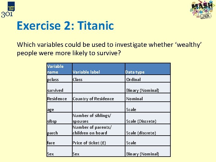
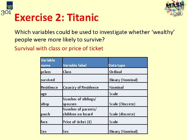
Exercise 2: Titanic Which variables could be used to investigate whether ‘wealthy’ people were more likely to survive? Variable name Variable label Data type pclass Class Ordinal survived Binary (Nominal) Residence Country of Residence Nominal age Scale parch Number of siblings/ spouses Number of parents/ children on board fare Price of ticket (£) Scale Sex Binary (Nominal) sibsp Scale (Discrete) Scale (discrete)

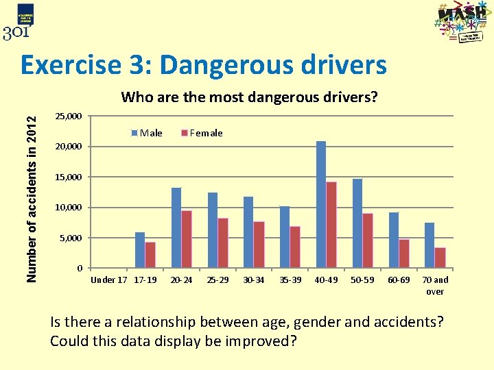
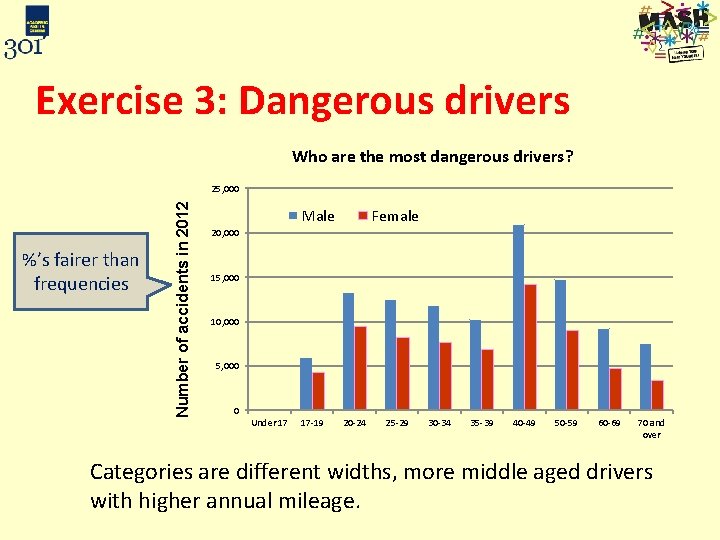
Exercise 3: Dangerous drivers Number of accidents in 2012 Who are the most dangerous drivers? 25, 000 Male Female 20, 000 15, 000 10, 000 5, 000 0 Under 17 17 -19 20 -24 25 -29 30 -34 35 -39 40 -49 50 -59 60 -69 70 and over Is there a relationship between age, gender and accidents? Could this data display be improved?

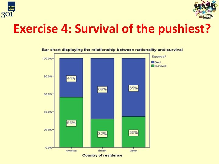
Exercise 4: Survival of the pushiest? • Are American’s more likely to survive when a boat sinks? Produce a suitable summary table and stacked barchart to investigate this http: //www. independent. co. uk/news/world/australasia/more-britons-than-americansdied-on-titanic-because-they-queued-1452299. html

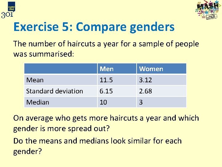
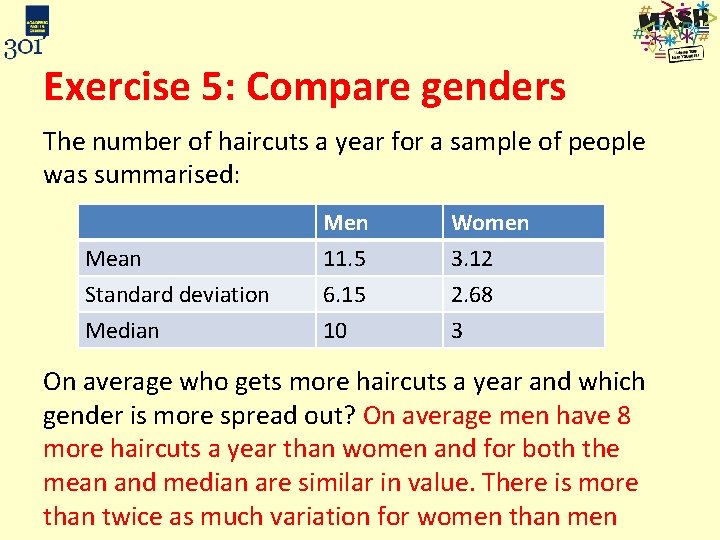
Exercise 5: Compare genders The number of haircuts a year for a sample of people was summarised: Mean Standard deviation Median Men 11. 5 6. 15 10 Women 3. 12 2. 68 3 On average who gets more haircuts a year and which gender is more spread out? Do the means and medians look similar for each gender?

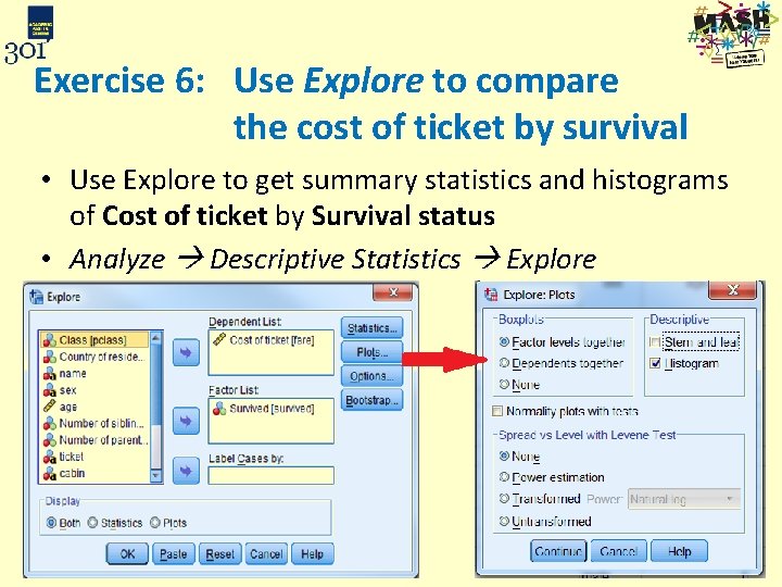
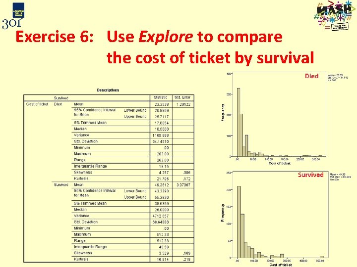
Exercise 6: Use Explore to compare the cost of ticket by survival • Use Explore to get summary statistics and histograms of Cost of ticket by Survival status • Analyze Descriptive Statistics Explore

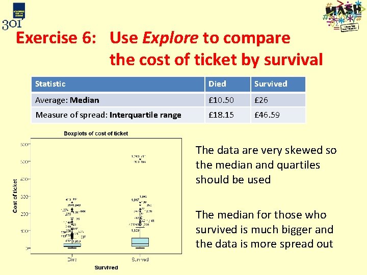
Exercise 6: Use Explore to compare the cost of ticket by survival • Which summary statistics should be used? • Interpret the output: how do the two groups (those who died and who survived) compare? • Use the histograms to decide which summary measures to use Statistic Average: Measure of spread: Died Survived

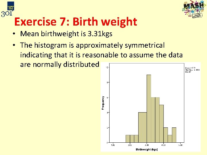
Exercise 7: Birth weight • Open up the ‘Birthweight_reduced’ spreadsheet from the EXCEL file • Give the variables suitable labels, including labels for the different levels of ‘lobwt’ and ‘mage 35’ • Recode mnocig ‘Number of cigarettes smoked per day’ into smoker/non-smoker • Use Automatic recode to convert ‘lowbwt’ from String to Numeric • Calculate the mean birth weight and produce a histogram. Is birth weight normally distributed or skewed?

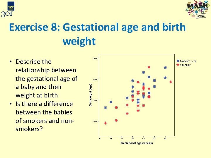
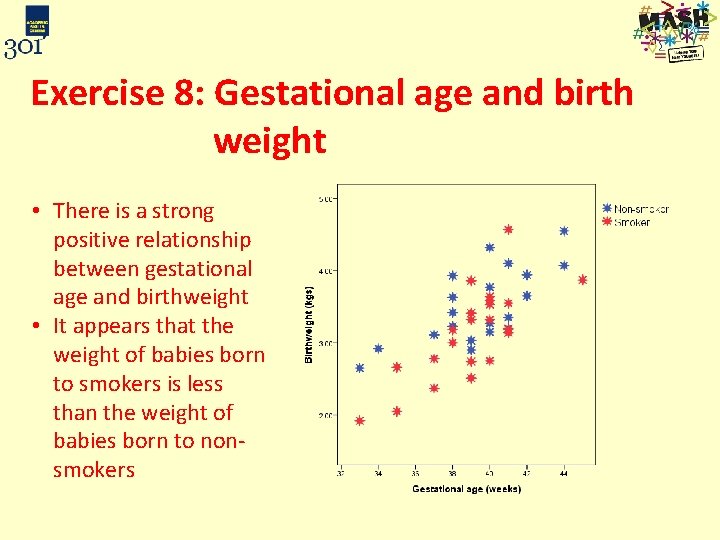
Exercise 8: Gestational age and birth weight • Describe the relationship between the gestational age of a baby and their weight at birth • Is there a difference between the babies of smokers and nonsmokers?

Additional exercise a) Open the file ‘Housework_mini’ b) Use suitable summary statistics and charts to see if there is a difference between the amount of housework carried out by men and women each week. c) Investigate the relationship between the amount of housework someone carries out per week and the hours they work using different markers for males and females. d) Create a new binary variable from ‘Hours worked per week’ to indicate whether someone is full time or part time. Classify part time as under 30 hours. e) Summarise the amount of housework carried out per week by working full/ part time using a table and a plot and interpret.

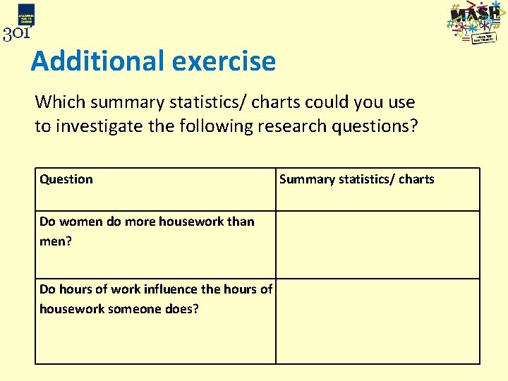
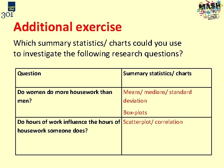
Additional exercise Which summary statistics/ charts could you use to investigate the following research questions? Question Summary statistics/ charts Do women do more housework than men? Do hours of work influence the hours of housework someone does?

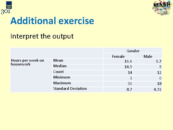
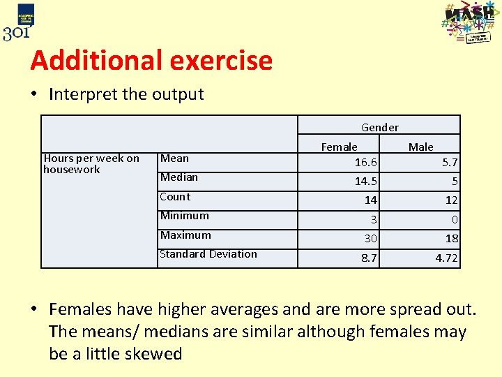
Additional exercise Interpret the output Hours per week on housework Gender Mean Median Count Minimum Maximum Standard Deviation Female 16. 6 14. 5 14 3 30 8. 7 Male 5. 7 5 12 0 18 4. 72

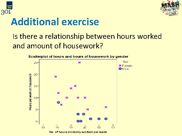
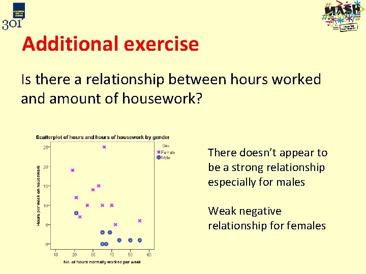
Additional exercise Is there a relationship between hours worked and amount of housework?

Exercise 2: Titanic Which variables could be used to investigate whether ‘wealthy’ people were more likely to survive? Survival with class or price of ticket Variable name Variable label Data type pclass Class Ordinal survived Binary (Nominal) Residence Country of Residence Nominal age Scale parch Number of siblings/ spouses Number of parents/ children on board fare Price of ticket (£) Scale Sex Binary (Nominal) sibsp Scale (Discrete) Scale (discrete)

Exercise 3: Dangerous drivers Who are the most dangerous drivers? %’s fairer than frequencies Number of accidents in 2012 25, 000 Male Female 20, 000 15, 000 10, 000 5, 000 0 Under 17 17 -19 20 -24 25 -29 30 -34 35 -39 40 -49 50 -59 60 -69 70 and over Categories are different widths, more middle aged drivers with higher annual mileage.

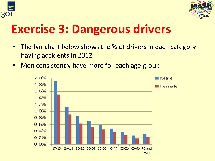
Exercise 3: Dangerous drivers • The bar chart below shows the % of drivers in each category having accidents in 2012 • Men consistently have more for each age group

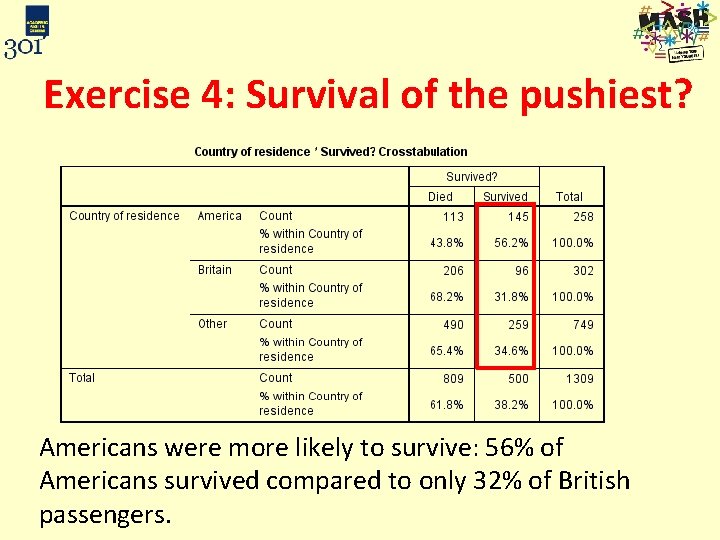
Exercise 4: Survival of the pushiest? Americans were more likely to survive: 56% of Americans survived compared to only 32% of British passengers.

Exercise 4: Survival of the pushiest?

Exercise 5: Compare genders The number of haircuts a year for a sample of people was summarised: Mean Standard deviation Median Men 11. 5 6. 15 10 Women 3. 12 2. 68 3 On average who gets more haircuts a year and which gender is more spread out? On average men have 8 more haircuts a year than women and for both the mean and median are similar in value. There is more than twice as much variation for women than men

Exercise 6: Use Explore to compare the cost of ticket by survival

Exercise 6: Use Explore to compare the cost of ticket by survival Statistic Died Survived Average: Median £ 10. 50 £ 26 Measure of spread: Interquartile range £ 18. 15 £ 46. 59 The data are very skewed so the median and quartiles should be used The median for those who survived is much bigger and the data is more spread out

Exercise 7: Birth weight • Mean birthweight is 3. 31 kgs • The histogram is approximately symmetrical indicating that it is reasonable to assume the data are normally distributed

Exercise 8: Gestational age and birth weight • There is a strong positive relationship between gestational age and birthweight • It appears that the weight of babies born to smokers is less than the weight of babies born to nonsmokers

Additional exercise Which summary statistics/ charts could you use to investigate the following research questions? Question Summary statistics/ charts Do women do more housework than men? Means/ medians/ standard deviation Box-plots Do hours of work influence the hours of Scatterplot/ correlation housework someone does?

Additional exercise • Interpret the output Gender Hours per week on housework Mean Median Count Minimum Maximum Standard Deviation Female 16. 6 Male 5. 7 14. 5 5 14 12 3 0 30 18 8. 7 4. 72 • Females have higher averages and are more spread out. The means/ medians are similar although females may be a little skewed

Additional exercise Is there a relationship between hours worked and amount of housework? There doesn’t appear to be a strong relationship especially for males Weak negative relationship for females

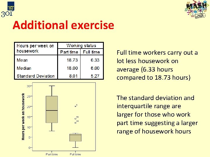
Additional exercise Full time workers carry out a lot less housework on average (6. 33 hours compared to 18. 73 hours) The standard deviation and interquartile range are larger for those who work part time suggesting a larger range of housework hours