Excel Power Query Power Query for Parsing Data

Data Models– Screen I 1 n Excel 2010 and 2013 need to install the

Data Models– Screen 25. The Transactions table has repeated items while the other two

Data Models– Screen 39. Foreign keys can have repeated data in the column you

Data Models– Screen 4 a. Flavors columns will act as the Primary key in

Data Models– Screen 510. Click in the Transactions table and click on the Insert

Data Models– Screen 611. In the Pivot Table Field List, click All and click

Data Models– Screen 712. Below the Transactions table on the Sheet 1 has extra

Parsing Data – Screen 1 1. Open 2 A. Parsing Text with Get &

Parsing Data – Screen 2 6. The Query Editor opens up and on the

Parsing Data – Screen 3 7. Click on Split Colum > By Delimiter >

Parsing Data – Screen 5 8. Now we want to parse out the. com.

Parsing Data – Screen 6 10. Click on Split Colum> By Delimiter > >

Parsing Data – Screen 7 10. Click on Split Colum> By Delimiter > >

Parsing Data – Screen 9 11. Click on Close & Load

Parsing Data – Screen 11 12. Below in the original table in Parse Text

Parsing Data – Screen 13 14. Right click on the Workbook Queries on the

Parsing Data – Screen 14 15. With the 2 rows added to the 37

Finding Duplicates – Screen 1 Find a list of people who are in both

Finding Duplicates – Screen 2 3. Click one table and click on Data Tab

Finding Duplicates – Screen 3 3. Click one table and click on Data Tab

Finding Duplicates – Screen 5 4. Right Click on the first table name in

Finding Duplicates – Screen 6 5. We need to choose the name of the

Finding Duplicates – Screen 7 5. We need to choose the name of the

Finding Duplicates – Screen 8 6. Click on Close & Load

Normalizing Tables– Screen 1 In order to pivot tables, sort tables, or filter tables;

Normalizing Tables– Screen 2 1. Open 4. Unpivot Example 2. Select the Table and

Normalizing Tables– Screen 4 5. Select the columns that need to be “unpivot” which

Normalizing Tables– Screen 6 8. Click on Close & Load

Normalizing Tables– Screen 8 9. Below in the original table in Sheet 1 has

Normalizing Tables– Screen 9 11. Right click on the Workbook Queries on the right

Normalizing Tables– Screen 10 12. With the 4 rows containing 10 months will convert

Power Query for Merging Tables with Empty Cells…

Merging Tables – Screen 1 When you need to consolidate multiple tables, let Power

Merging Tables – Screen 2 4. Select each table and click on Data Tab

Merging Tables – Screen 3 4. Select each table and click on Data Tab

Merging Tables – Screen 4 The Workbook Queries has the four tables with Connection

Merging Tables – Screen 5 7. Right click in the Workbook Queries pane the

Merging Tables – Screen 6 8. Choose Three or more tables.

Merging Tables – Screen 7 9. Add the other three tables to the right

Merging Tables – Screen 8 11. Click on Close & Load • The North.

Flash Fill Make sure that your Flash Fill is activated. Go to File >

Flash Fill Tips • To use Flash Fill you need to be in the

Slides: 69

Download presentation

Excel Power Query

Power Query for Parsing Data…

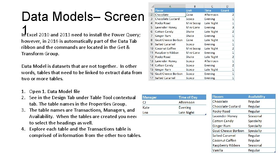
Data Models– Screen I 1 n Excel 2010 and 2013 need to install the Power Query; however, in 2016 is automatically part of the Data Tab ribbon and the commands are located in the Get & Transform Group. Data Model is datasets that are not together. In other words, tables that need to be linked to extract data from two or more tables. 1. Open 1. Data Model file 2. See in the Design Tab under Table Tool contextual tab. The table names in the Properties Group. 3. The table names are Transactions, Managers, and Availability. When the tables are created you need to select the headings as well. 4. Explore each table and the Transactions table is comprised of information from the other two tables.

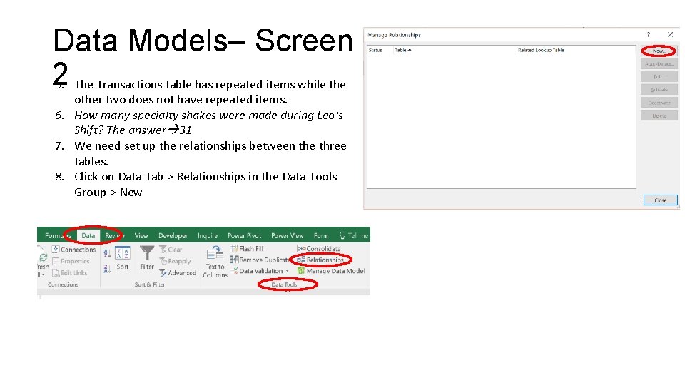
Data Models– Screen 25. The Transactions table has repeated items while the other two does not have repeated items. 6. How many specialty shakes were made during Leo's Shift? The answer 31 7. We need set up the relationships between the three tables. 8. Click on Data Tab > Relationships in the Data Tools Group > New

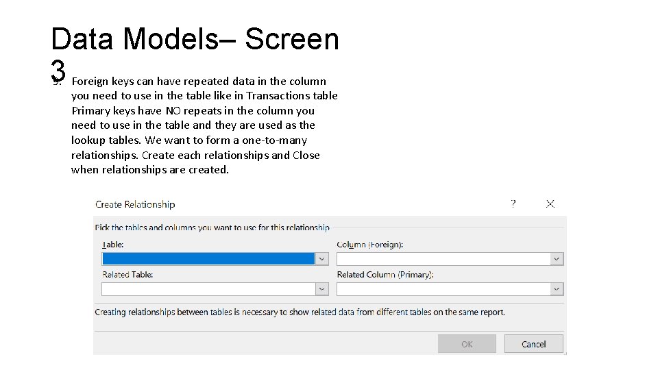
Data Models– Screen 39. Foreign keys can have repeated data in the column you need to use in the table like in Transactions table Primary keys have NO repeats in the column you need to use in the table and they are used as the lookup tables. We want to form a one-to-many relationships. Create each relationships and Close when relationships are created.

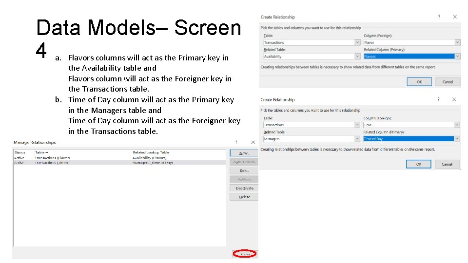
Data Models– Screen 4 a. Flavors columns will act as the Primary key in the Availability table and Flavors column will act as the Foreigner key in the Transactions table. b. Time of Day column will act as the Primary key in the Managers table and Time of Day column will act as the Foreigner key in the Transactions table.

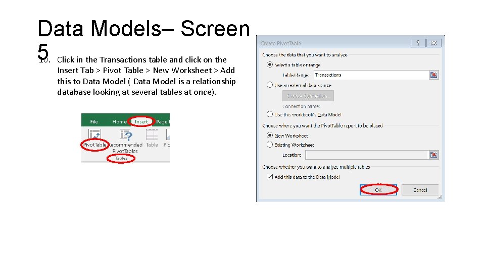
Data Models– Screen 510. Click in the Transactions table and click on the Insert Tab > Pivot Table > New Worksheet > Add this to Data Model ( Data Model is a relationship database looking at several tables at once).

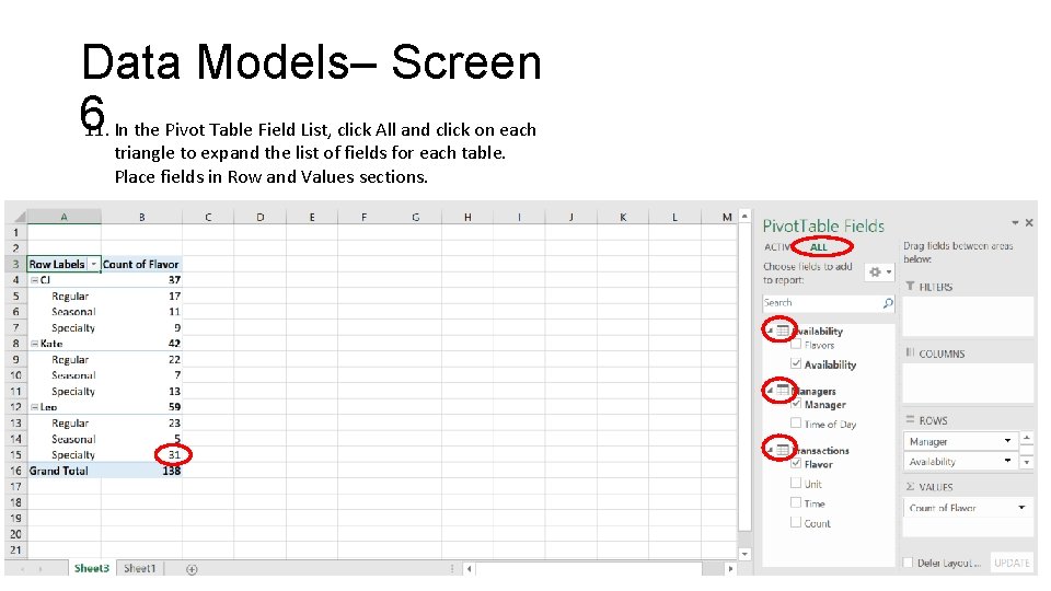
Data Models– Screen 611. In the Pivot Table Field List, click All and click on each triangle to expand the list of fields for each table. Place fields in Row and Values sections.

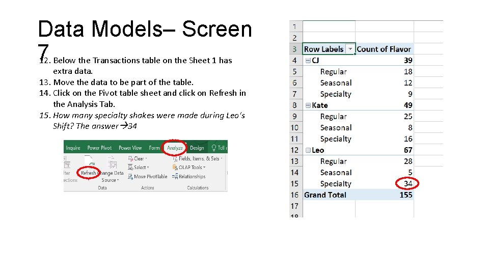
Data Models– Screen 712. Below the Transactions table on the Sheet 1 has extra data. 13. Move the data to be part of the table. 14. Click on the Pivot table sheet and click on Refresh in the Analysis Tab. 15. How many specialty shakes were made during Leo's Shift? The answer 34

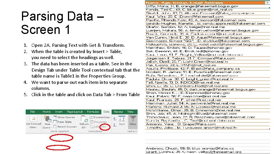
Parsing Data – Screen 1 1. Open 2 A. Parsing Text with Get & Transform. 2. When the table is created by Insert > Table, you need to select the headings as well. 3. The data has been inserted as a table. See in the Design Tab under Table Tool contextual tab that the table name is Table 1 in the Properties Group. 4. We want to parse out each item into separate columns. 5. Click in the table and click on Data Tab > From Table

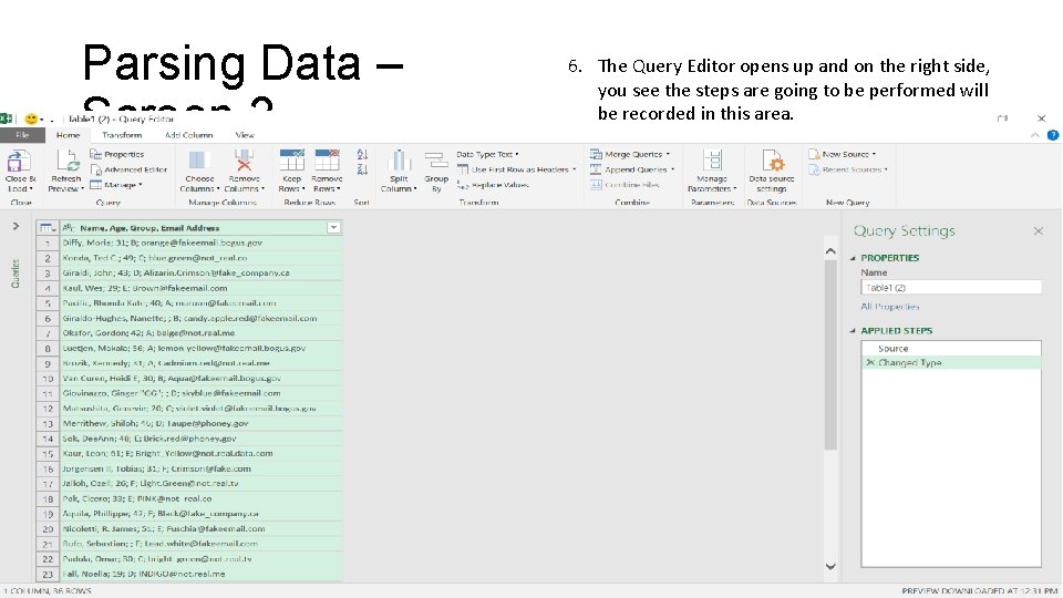
Parsing Data – Screen 2 6. The Query Editor opens up and on the right side, you see the steps are going to be performed will be recorded in this area.

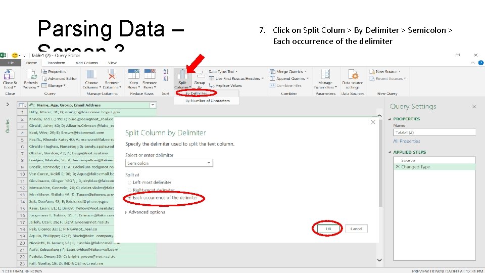
Parsing Data – Screen 3 7. Click on Split Colum > By Delimiter > Semicolon > Each occurrence of the delimiter

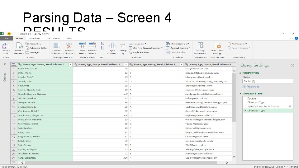
Parsing Data – Screen 4 RESULTS

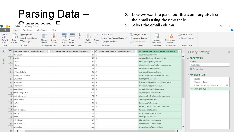
Parsing Data – Screen 5 8. Now we want to parse out the. com. org etc. from the emails using the new table. 9. Select the email column.

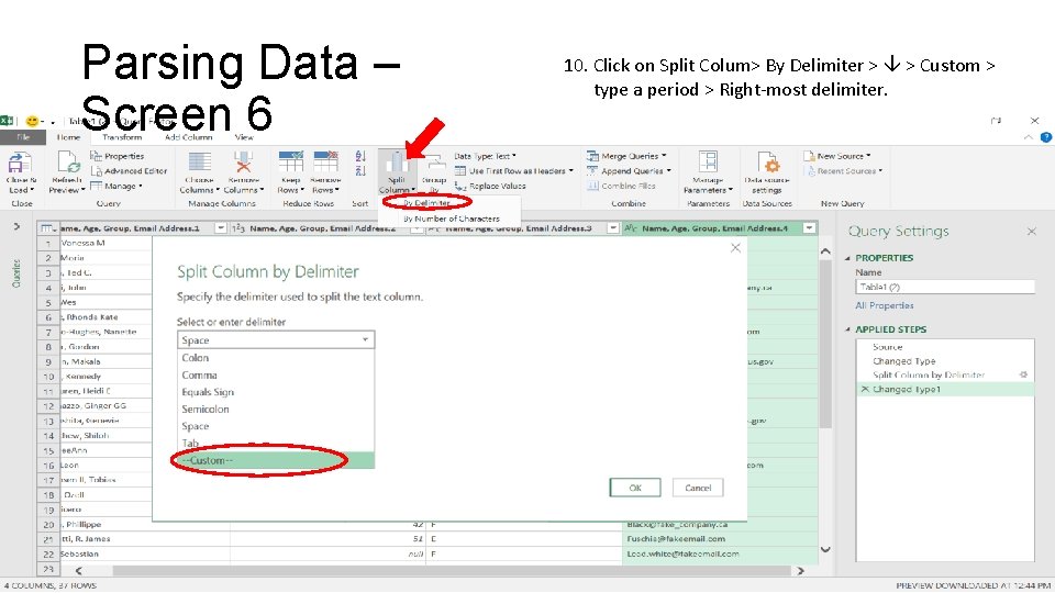
Parsing Data – Screen 6 10. Click on Split Colum> By Delimiter > > Custom > type a period > Right-most delimiter.

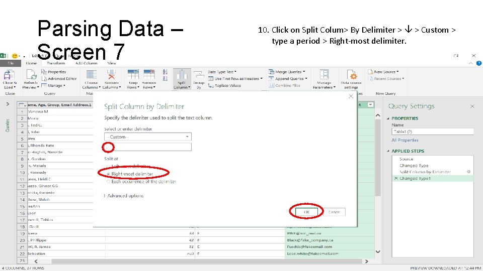
Parsing Data – Screen 7 10. Click on Split Colum> By Delimiter > > Custom > type a period > Right-most delimiter.

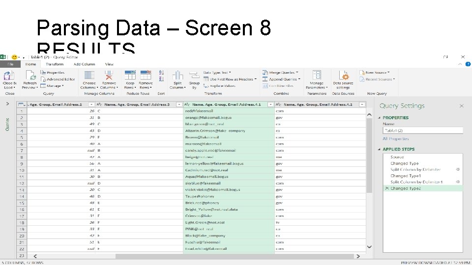
Parsing Data – Screen 8 RESULTS

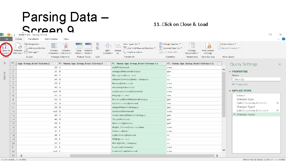
Parsing Data – Screen 9 11. Click on Close & Load

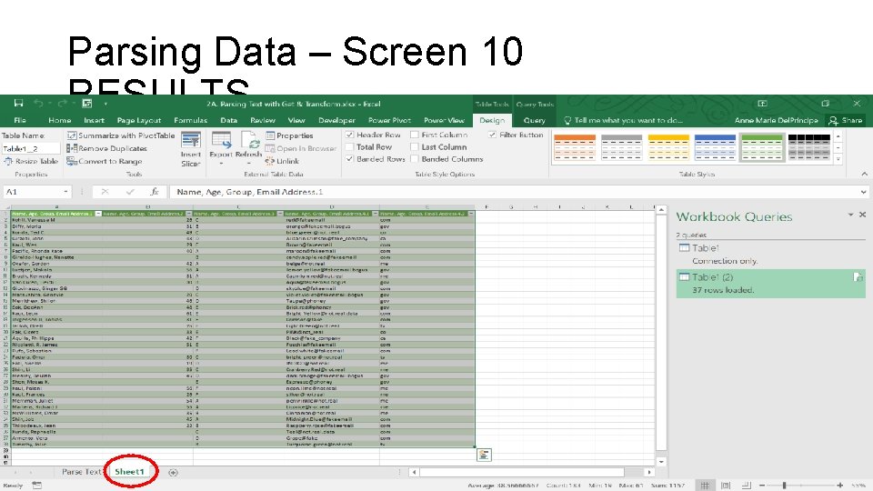
Parsing Data – Screen 10 RESULTS

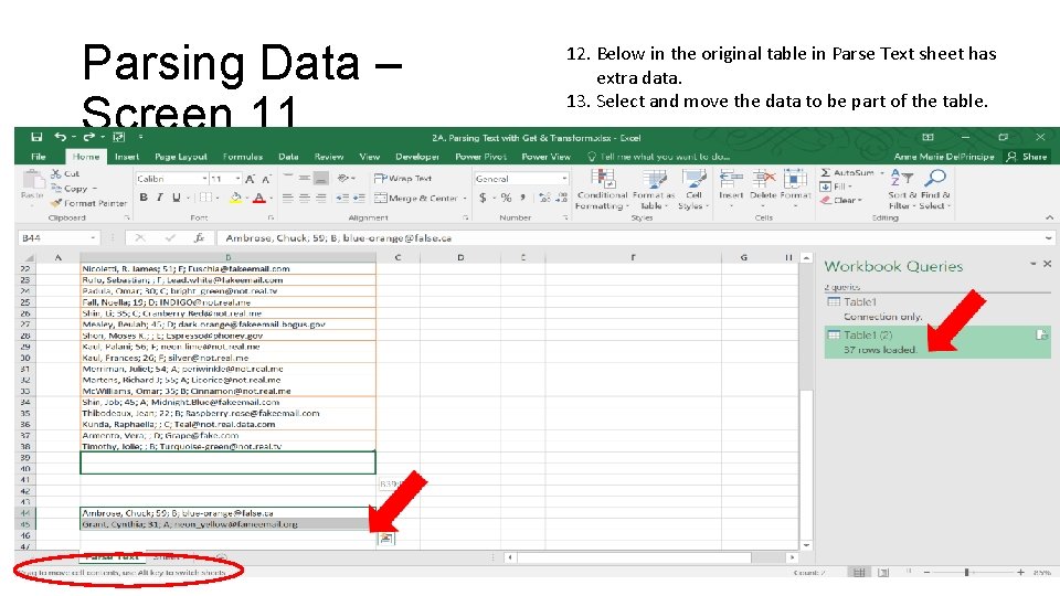
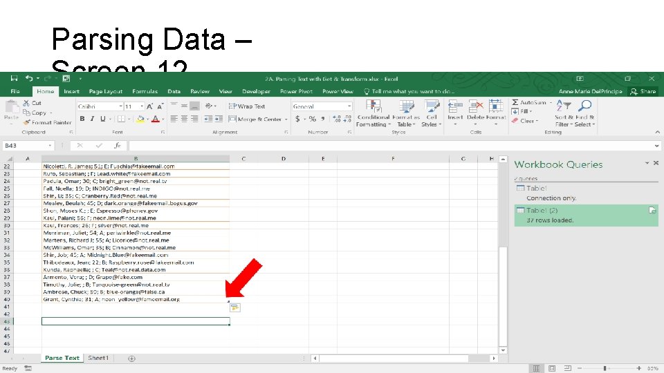
Parsing Data – Screen 11 12. Below in the original table in Parse Text sheet has extra data. 13. Select and move the data to be part of the table.

Parsing Data – Screen 12

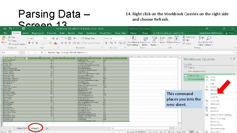
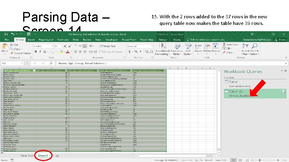
Parsing Data – Screen 13 14. Right click on the Workbook Queries on the right side and choose Refresh. This command places you into the new sheet.

Parsing Data – Screen 14 15. With the 2 rows added to the 37 rows in the new query table now makes the table have 39 rows.

Power Query for Finding Duplicates…

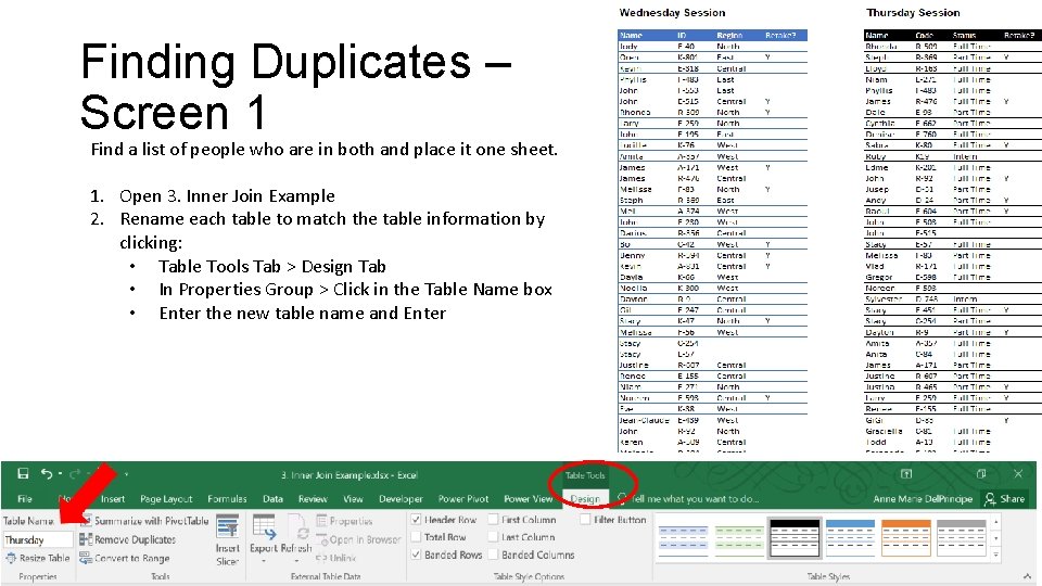
Finding Duplicates – Screen 1 Find a list of people who are in both and place it one sheet. 1. Open 3. Inner Join Example 2. Rename each table to match the table information by clicking: • Table Tools Tab > Design Tab • In Properties Group > Click in the Table Name box • Enter the new table name and Enter

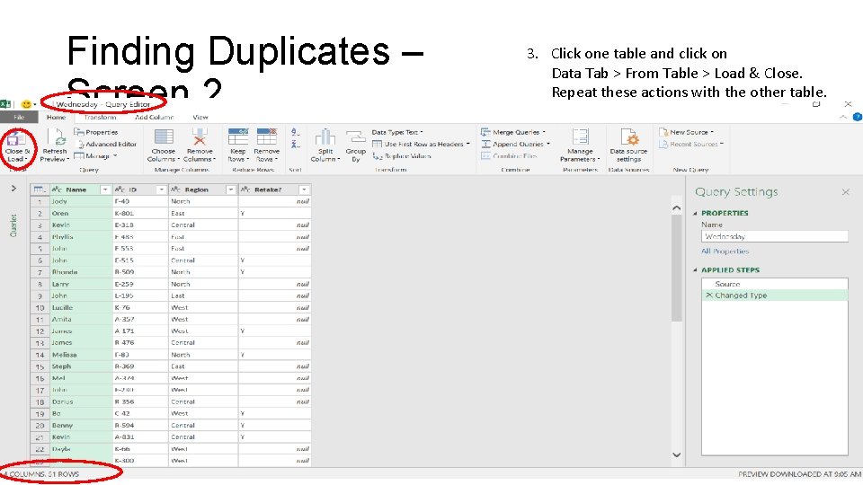
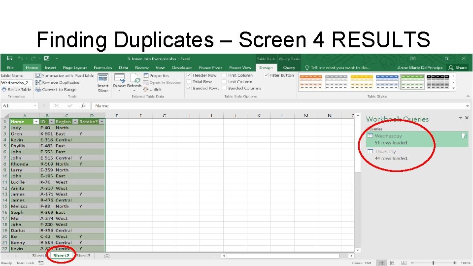
Finding Duplicates – Screen 2 3. Click one table and click on Data Tab > From Table > Load & Close. Repeat these actions with the other table.

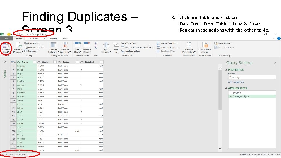
Finding Duplicates – Screen 3 3. Click one table and click on Data Tab > From Table > Load & Close. Repeat these actions with the other table.

Finding Duplicates – Screen 4 RESULTS

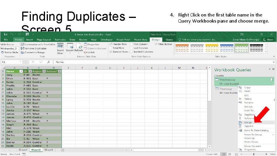
Finding Duplicates – Screen 5 4. Right Click on the first table name in the Query Workbooks pane and choose merge.

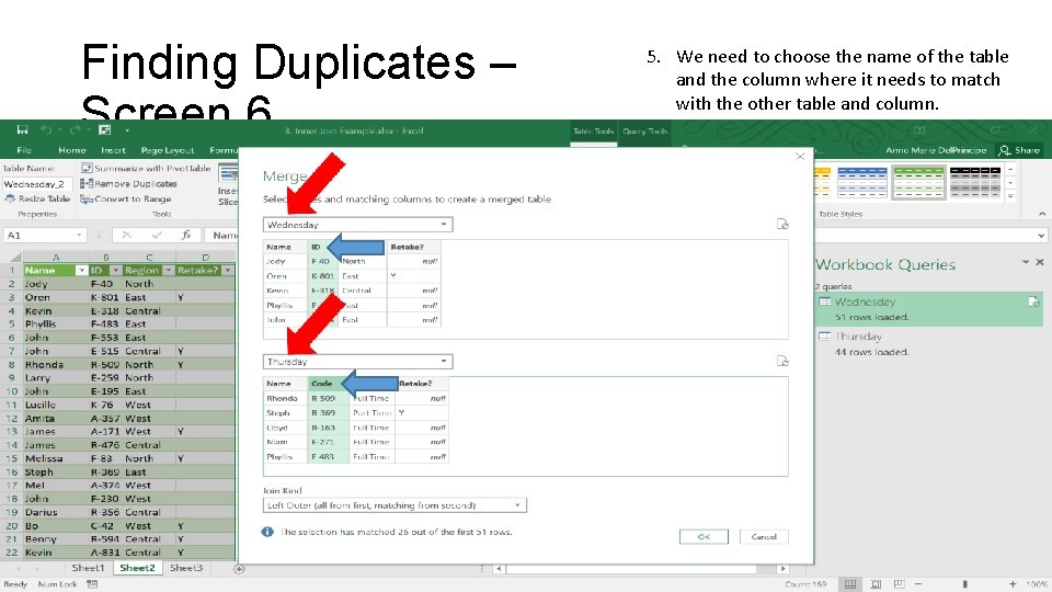
Finding Duplicates – Screen 6 5. We need to choose the name of the table and the column where it needs to match with the other table and column.

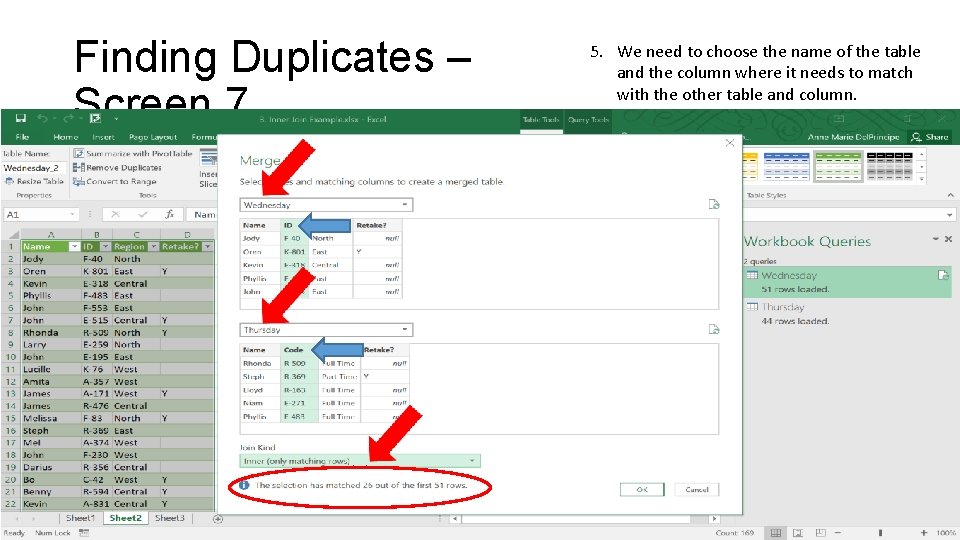
Finding Duplicates – Screen 7 5. We need to choose the name of the table and the column where it needs to match with the other table and column.

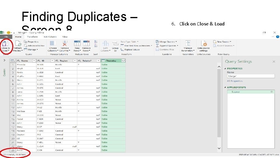
Finding Duplicates – Screen 8 6. Click on Close & Load

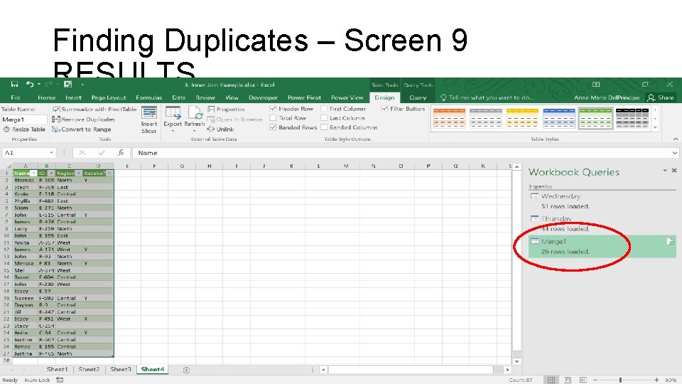
Finding Duplicates – Screen 9 RESULTS

Power Query for Normalizing Tables…

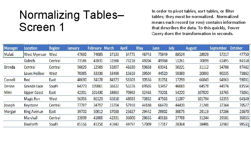
Normalizing Tables– Screen 1 In order to pivot tables, sort tables, or filter tables; they must be normalized. Normalized means each record (or row) contains information that describes the data. To this quickly, Power Query does the transformation in seconds.

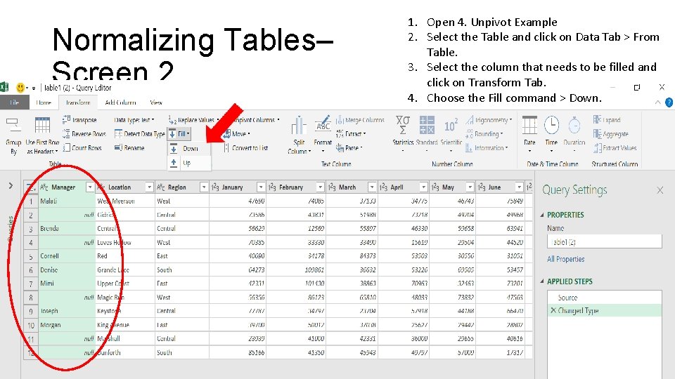
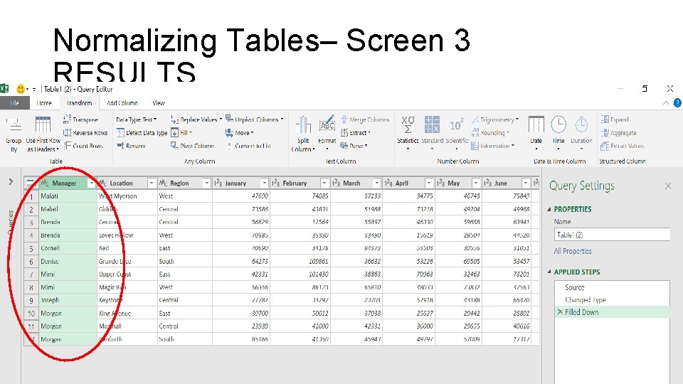
Normalizing Tables– Screen 2 1. Open 4. Unpivot Example 2. Select the Table and click on Data Tab > From Table. 3. Select the column that needs to be filled and click on Transform Tab. 4. Choose the Fill command > Down.

Normalizing Tables– Screen 3 RESULTS

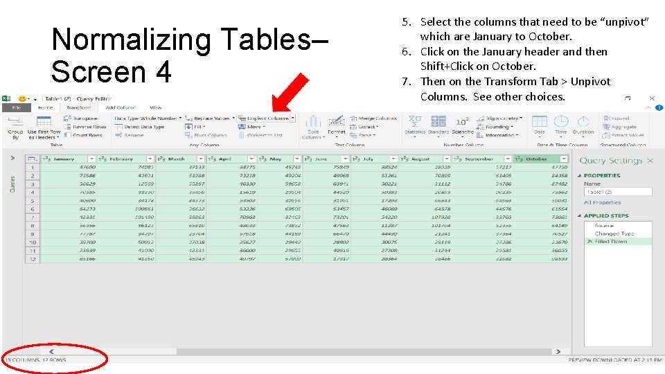
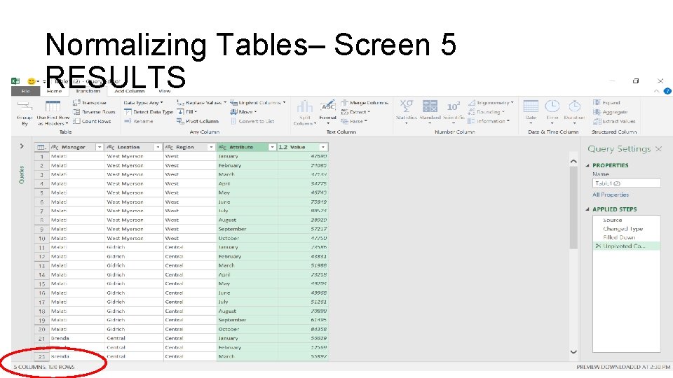
Normalizing Tables– Screen 4 5. Select the columns that need to be “unpivot” which are January to October. 6. Click on the January header and then Shift+Click on October. 7. Then on the Transform Tab > Unpivot Columns. See other choices.

Normalizing Tables– Screen 5 RESULTS

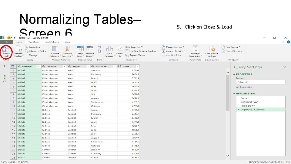
Normalizing Tables– Screen 6 8. Click on Close & Load

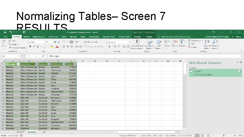
Normalizing Tables– Screen 7 RESULTS

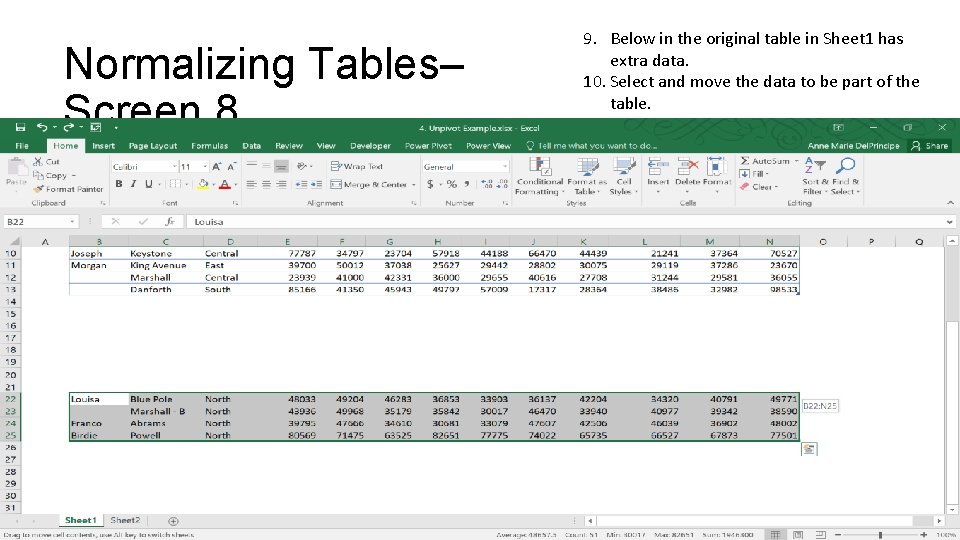
Normalizing Tables– Screen 8 9. Below in the original table in Sheet 1 has extra data. 10. Select and move the data to be part of the table.

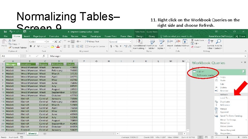
Normalizing Tables– Screen 9 11. Right click on the Workbook Queries on the right side and choose Refresh.

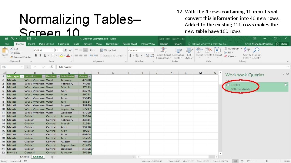
Normalizing Tables– Screen 10 12. With the 4 rows containing 10 months will convert this information into 40 new rows. Added to the existing 120 rows makes the new table have 160 rows.

Power Query for Merging Tables with Empty Cells…

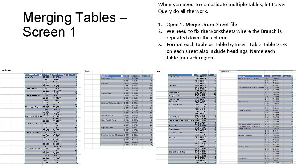
Merging Tables – Screen 1 When you need to consolidate multiple tables, let Power Query do all the work. 1. Open 5. Merge Order Sheet file 2. We need to fix the worksheets where the Branch is repeated down the column. 3. Format each table as Table by Insert Tab > Table > OK on each sheet also include headings. Name each table for each region.

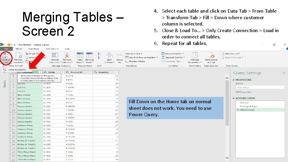
Merging Tables – Screen 2 4. Select each table and click on Data Tab > From Table > Transform Tab > Fill > Down where customer column is selected. 5. Close & Load To… > Only Create Connection > Load in order to connect all tables. 6. Repeat for all tables. Fill Down on the Home tab on normal sheet does not work. You need to use Power Query.

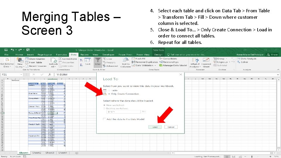
Merging Tables – Screen 3 4. Select each table and click on Data Tab > From Table > Transform Tab > Fill > Down where customer column is selected. 5. Close & Load To… > Only Create Connection > Load in order to connect all tables. 6. Repeat for all tables.

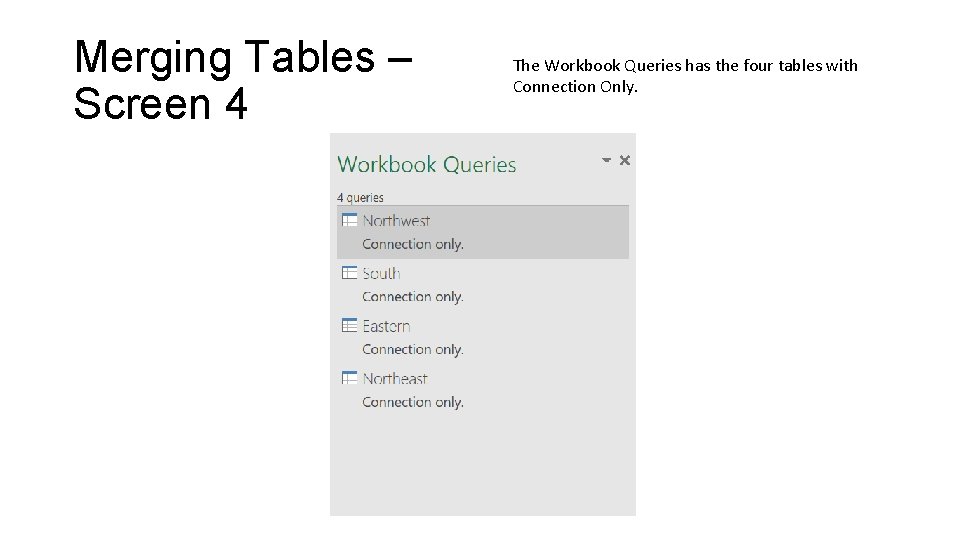
Merging Tables – Screen 4 The Workbook Queries has the four tables with Connection Only.

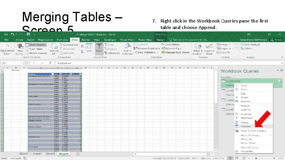
Merging Tables – Screen 5 7. Right click in the Workbook Queries pane the first table and choose Append.

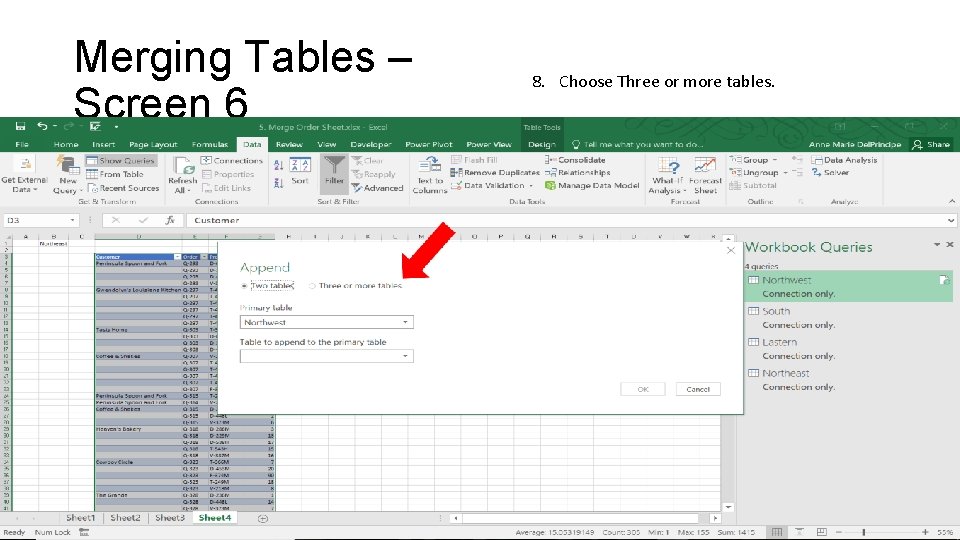
Merging Tables – Screen 6 8. Choose Three or more tables.

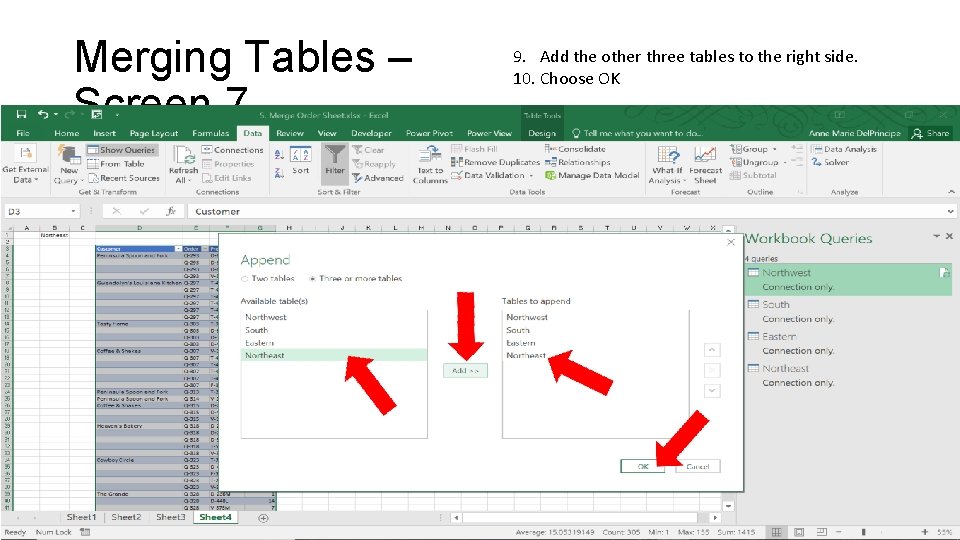
Merging Tables – Screen 7 9. Add the other three tables to the right side. 10. Choose OK

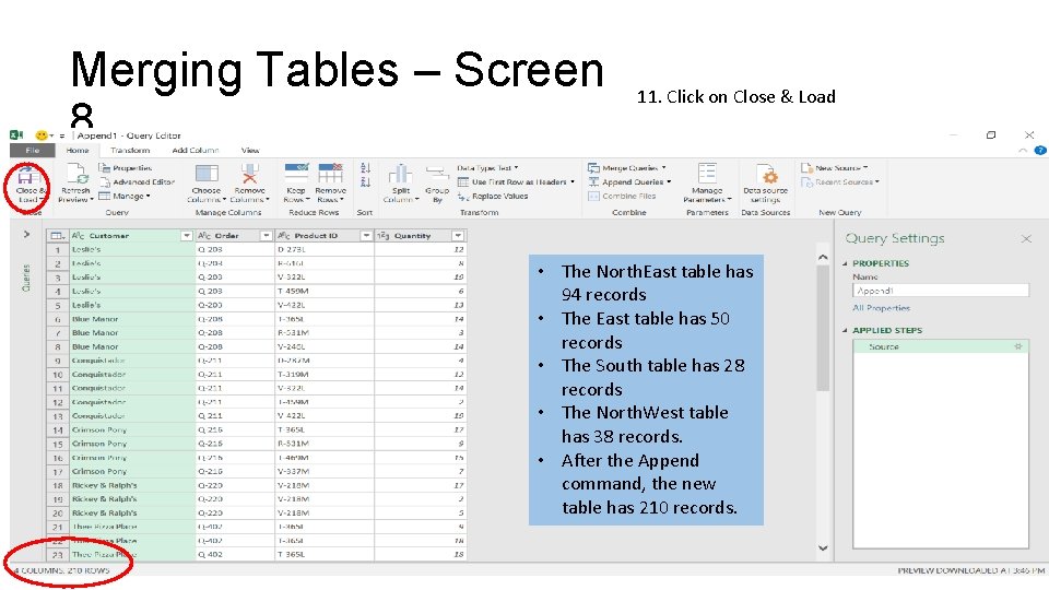
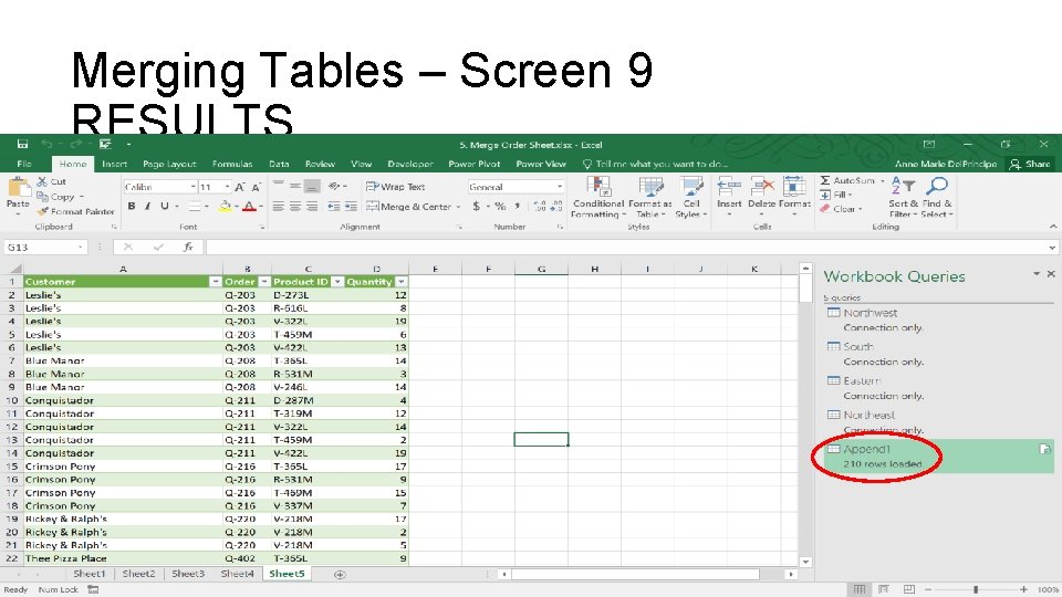
Merging Tables – Screen 8 11. Click on Close & Load • The North. East table has 94 records • The East table has 50 records • The South table has 28 records • The North. West table has 38 records. • After the Append command, the new table has 210 records.

Merging Tables – Screen 9 RESULTS

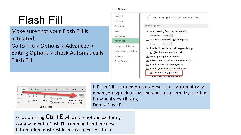
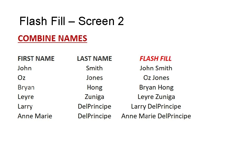
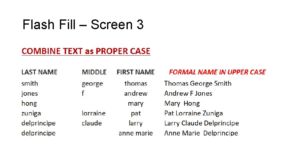
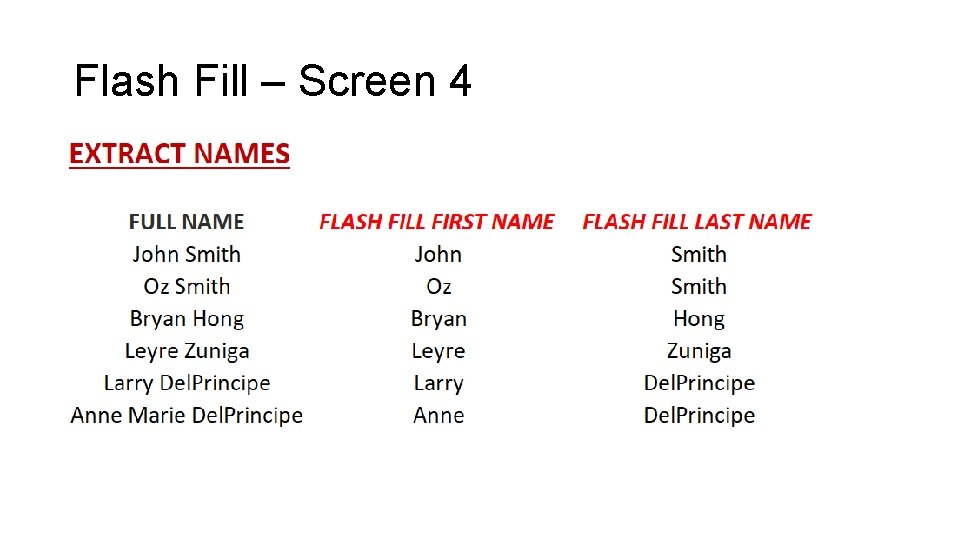
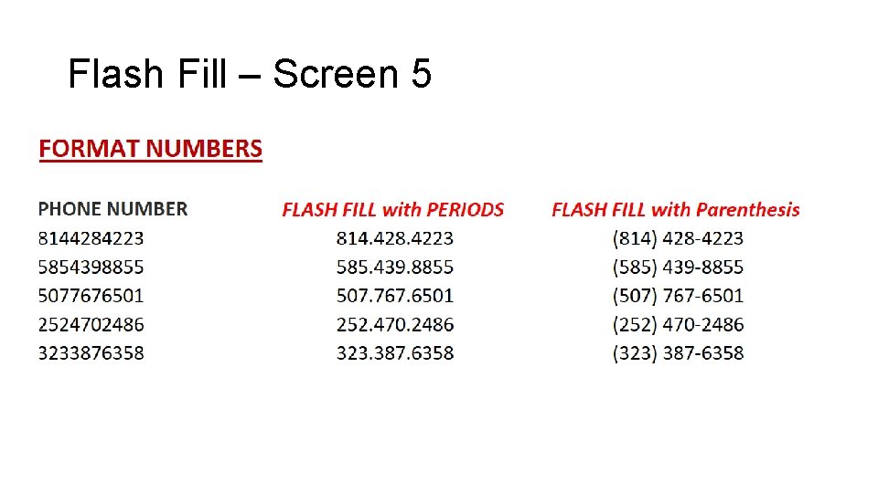
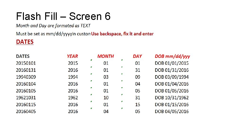
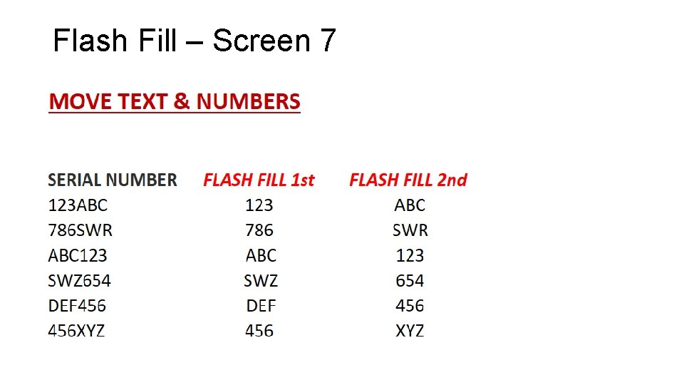
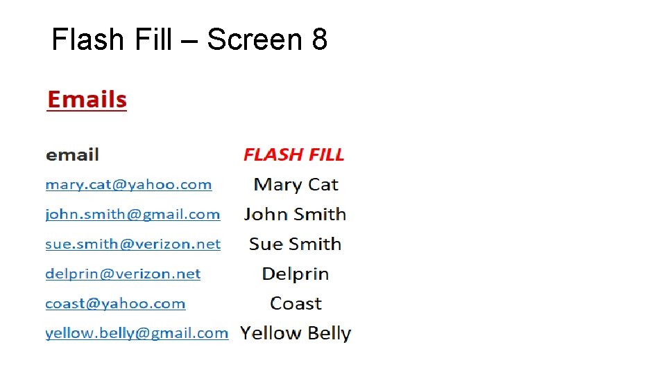
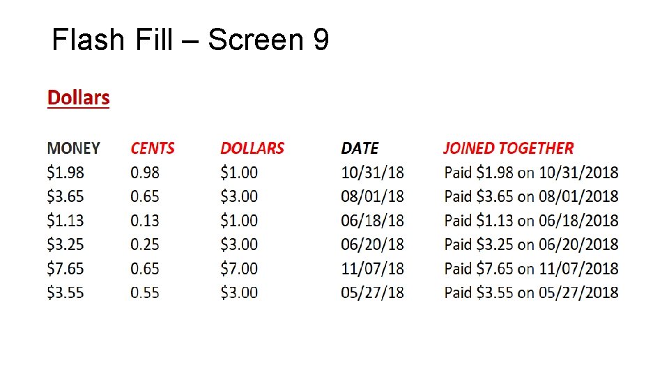
Flash Fill Make sure that your Flash Fill is activated. Go to File > Options > Advanced > Editing Options > check Automatically Flash Fill. If Flash Fill is turned on but doesn’t start automatically when you type data that matches a pattern, try starting it manually by clicking Data > Flash Fill or by pressing Ctrl+E which it is not the centering command but a Flash Fill command the new information must reside in a cell next to a table.

Excel Flash Fill

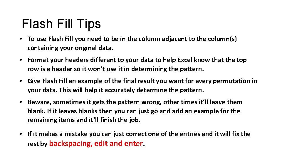
Flash Fill Tips • To use Flash Fill you need to be in the column adjacent to the column(s) containing your original data. • Format your headers different to your data to help Excel know that the top row is a header so it won’t use it in determining the pattern. • Give Flash Fill an example of the final result you want for every permutation in your data. This will help it accurately determine the pattern. • Beware, sometimes it gets the pattern wrong, other times it’ll leave them blank. If it leaves blanks then you can just go and add an example for the remaining items and it’ll finish the job. • If it makes a mistake you can just correct one of the entries and it will fix the rest by backspacing, edit and enter.

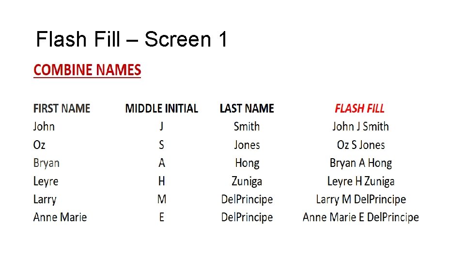
Flash Fill – Screen 1

Flash Fill – Screen 2

Flash Fill – Screen 3

Flash Fill – Screen 4

Flash Fill – Screen 5

Flash Fill – Screen 6

Flash Fill – Screen 7

Flash Fill – Screen 8

Flash Fill – Screen 9

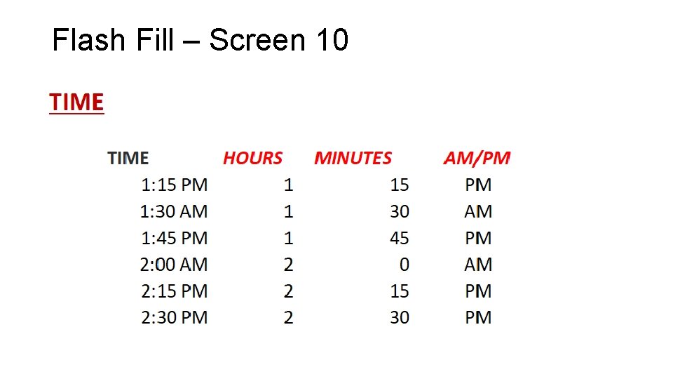
Flash Fill – Screen 10

Thank You