Excel Pivot Tabl es SOUTH HILLS SCHOOL OF

Excel Pivot. Tabl es SOUTH HILLS SCHOOL OF BUSINESS & TECHNOLOGY Express Excel Session April 27, 2020 Presenter: Marsha Ann Tate, Ph. D.

Topics to be Covered v What is a Pivot. Table? v Common Uses of Pivot. Tables v Create a Recommended Pivot. Table v Areas of a Pivot. Table v Modifying a Pivot. Table

Pivot. Table “[A] dynamic data table…that you can manipulate to emphasize different views of a data list stored in Excel” (Frye). “[U]ses calculations to consolidate and summarize data” (Poatsy, 339).

Pivot. Table Uses Ø Allows analysis of data from a data source without altering the original dataset. Ø Data can be quickly and easily rearranged for analysis from different viewpoints.

Preparation of the Data Source Before you create a Pivot. Table, your data source must: Ø Use unique and descriptive column labels Ø Not contain any blank rows or columns Ø Include at least one column with duplicate values (e. g. , the same town or department name) ØThis is needed to generate categories for organizing and summarizing data.

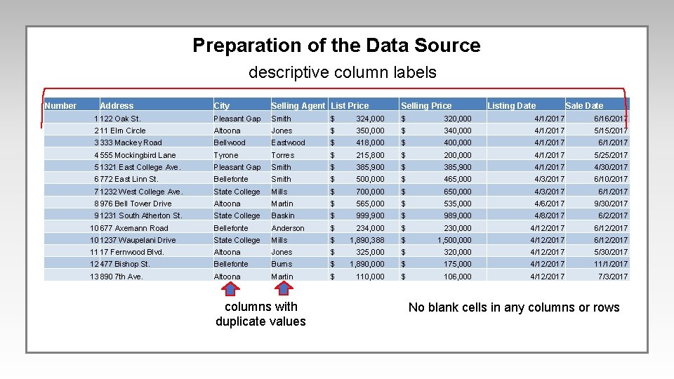
Preparation of the Data Source descriptive column labels Number Address City Selling Agent List Price Selling Price 1 122 Oak St. Pleasant Gap Smith $ 324, 000 $ 320, 000 4/1/2017 6/16/2017 2 11 Elm Circle Altoona Jones $ 350, 000 $ 340, 000 4/1/2017 5/15/2017 3 333 Mackey Road Bellwood Eastwood $ 418, 000 $ 400, 000 4/1/2017 6/1/2017 4 555 Mockingbird Lane Tyrone Torres $ 215, 800 $ 200, 000 4/1/2017 5/25/2017 5 1321 East College Ave. Pleasant Gap Smith $ 385, 900 4/1/2017 4/30/2017 6 772 East Linn St. Bellefonte Smith $ 500, 000 $ 465, 000 4/3/2017 6/10/2017 7 1232 West College Ave. State College Mills $ 700, 000 $ 650, 000 4/3/2017 6/1/2017 8 976 Bell Tower Drive Altoona Martin $ 565, 000 $ 535, 000 4/6/2017 9/30/2017 9 1231 South Atherton St. State College Baskin $ 999, 900 $ 989, 000 4/8/2017 6/2/2017 10 677 Axemann Road Bellefonte Anderson $ 234, 000 $ 230, 000 4/12/2017 6/12/2017 10 1237 Waupelani Drive State College Mills $ 1, 890, 388 $ 1, 500, 000 4/12/2017 6/12/2017 11 17 Fernwood Blvd. Altoona Jones $ 325, 000 $ 320, 000 4/12/2017 5/30/2017 12 477 Bishop St. Bellefonte Burns $ 1, 890, 000 $ 175, 000 4/12/2017 11/1/2017 13 890 7 th Ave. Altoona Martin $ 110, 000 $ 106, 000 4/12/2017 7/3/2017 columns with duplicate values Listing Date Sale Date No blank cells in any columns or rows

Create Pivot. Tables Using Quick Analysis and Recommended Pivot. Tables

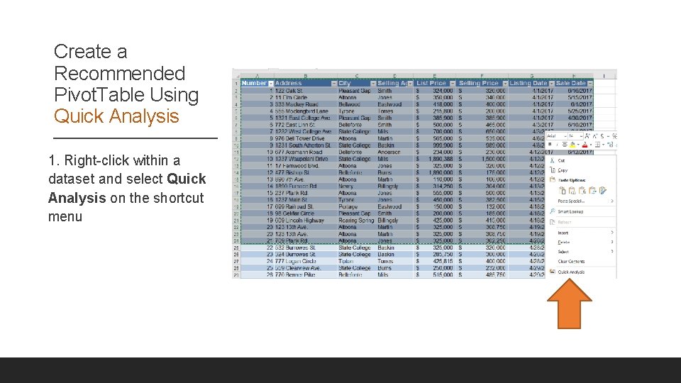
Create a Recommended Pivot. Table Using Quick Analysis 1. Right-click within a dataset and select Quick Analysis on the shortcut menu

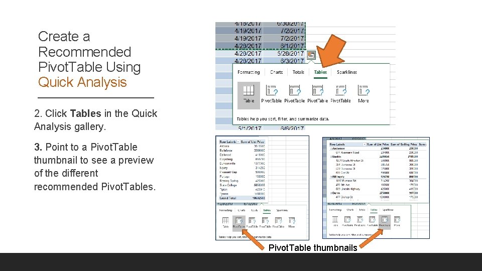
Create a Recommended Pivot. Table Using Quick Analysis 2. Click Tables in the Quick Analysis gallery. 3. Point to a Pivot. Table thumbnail to see a preview of the different recommended Pivot. Tables. Pivot. Table thumbnails

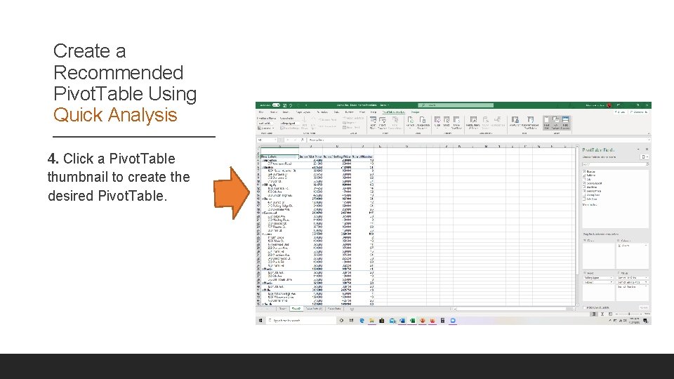
Create a Recommended Pivot. Table Using Quick Analysis 4. Click a Pivot. Table thumbnail to create the desired Pivot. Table.

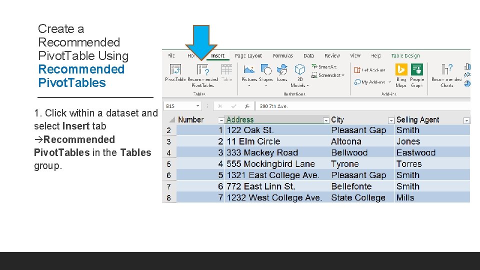
Create a Recommended Pivot. Table Using Recommended Pivot. Tables 1. Click within a dataset and select Insert tab Recommended Pivot. Tables in the Tables group.

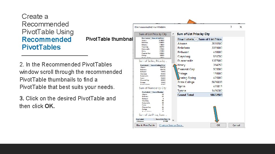
Create a Recommended Pivot. Table Using Recommended Pivot. Tables Pivot. Table thumbnails 2. In the Recommended Pivot. Tables window scroll through the recommended Pivot. Table thumbnails to find a Pivot. Table that best suits your needs. 3. Click on the desired Pivot. Table and then click OK.

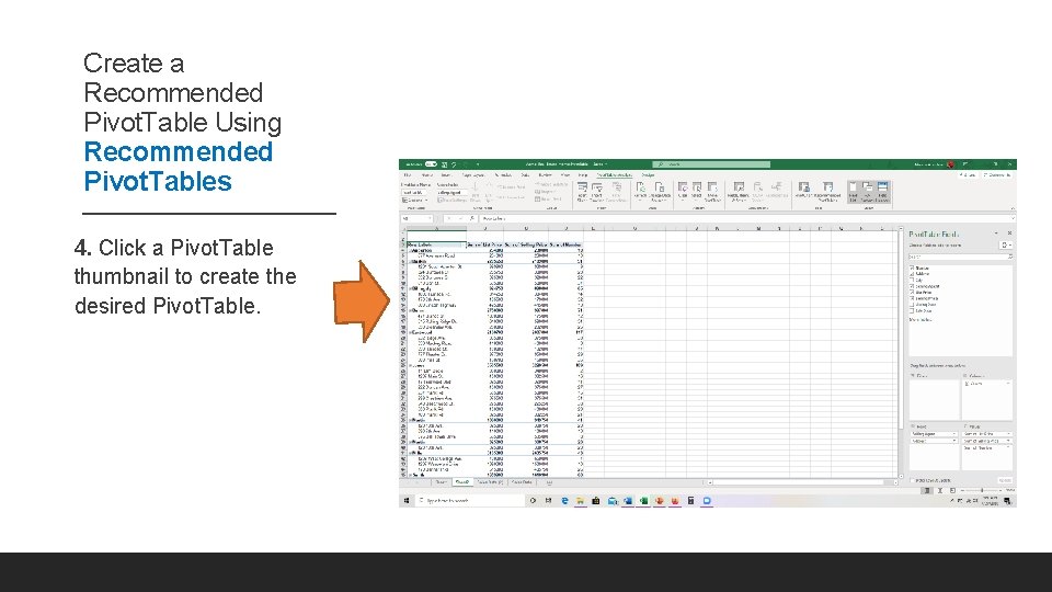
Create a Recommended Pivot. Table Using Recommended Pivot. Tables 4. Click a Pivot. Table thumbnail to create the desired Pivot. Table.

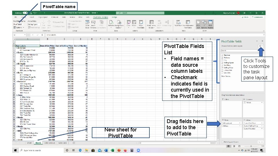
Pivot. Table name Pivot. Table Fields List • Field names = data source column labels • Checkmark indicates field is currently used in the Pivot. Table New sheet for Pivot. Table Drag fields here to add to the Pivot. Table Click Tools to customize the task pane layout

Pivot. Table Sections

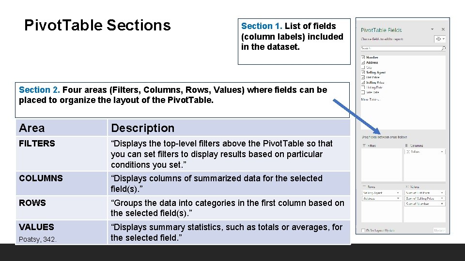
Pivot. Table Sections Section 1. List of fields (column labels) included in the dataset. Section 2. Four areas (Filters, Columns, Rows, Values) where fields can be placed to organize the layout of the Pivot. Table. Area Description FILTERS “Displays the top-level filters above the Pivot. Table so that you can set filters to display results based on particular conditions you set. ” COLUMNS “Displays columns of summarized data for the selected field(s). ” ROWS “Groups the data into categories in the first column based on the selected field(s). ” VALUES “Displays summary statistics, such as totals or averages, for the selected field. ” Poatsy, 342.

Modifying a Pivot. Table

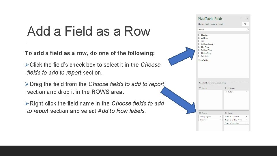
Add a Field as a Row To add a field as a row, do one of the following: ØClick the field’s check box to select it in the Choose fields to add to report section. ØDrag the field from the Choose fields to add to report section and drop it in the ROWS area. ØRight-click the field name in the Choose fields to add to report section and select Add to Row labels.

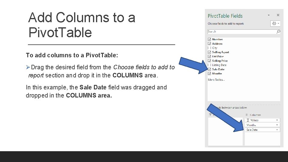
Add Columns to a Pivot. Table To add columns to a Pivot. Table: ØDrag the desired field from the Choose fields to add to report section and drop it in the COLUMNS area. In this example, the Sale Date field was dragged and dropped in the COLUMNS area.

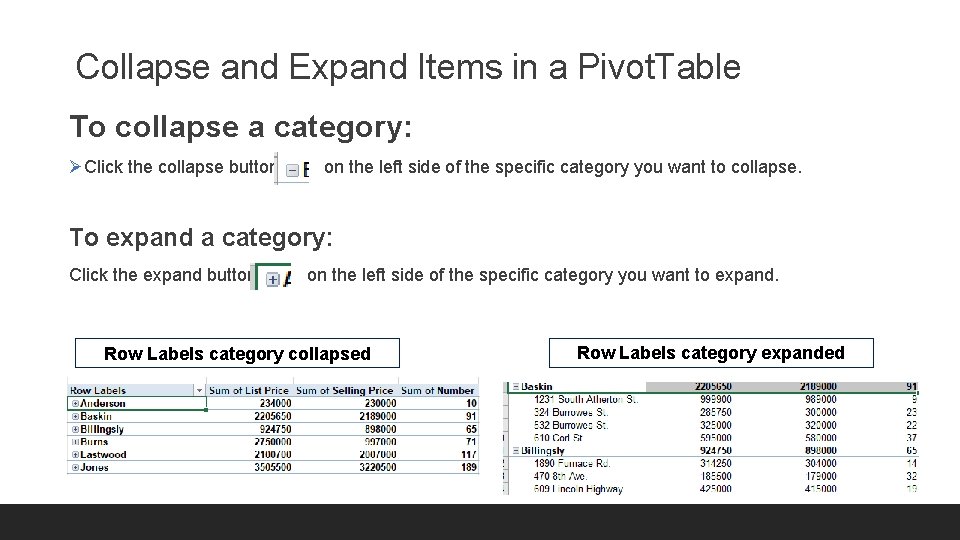
Collapse and Expand Items in a Pivot. Table To collapse a category: ØClick the collapse button on the left side of the specific category you want to collapse. To expand a category: Click the expand button on the left side of the specific category you want to expand. Row Labels category collapsed Row Labels category expanded

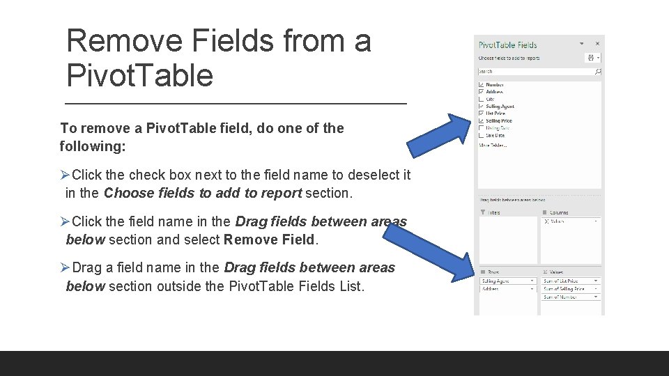
Remove Fields from a Pivot. Table To remove a Pivot. Table field, do one of the following: ØClick the check box next to the field name to deselect it in the Choose fields to add to report section. ØClick the field name in the Drag fields between areas below section and select Remove Field. ØDrag a field name in the Drag fields between areas below section outside the Pivot. Table Fields List.

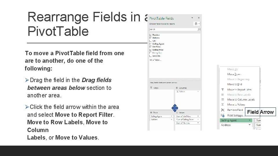
Rearrange Fields in a Pivot. Table To move a Pivot. Table field from one are to another, do one of the following: ØDrag the field in the Drag fields between areas below section to another area. ØClick the field arrow within the area and select Move to Report Filter. Move to Row Labels, Move to Column Labels, or Move to Values. Field Arrow

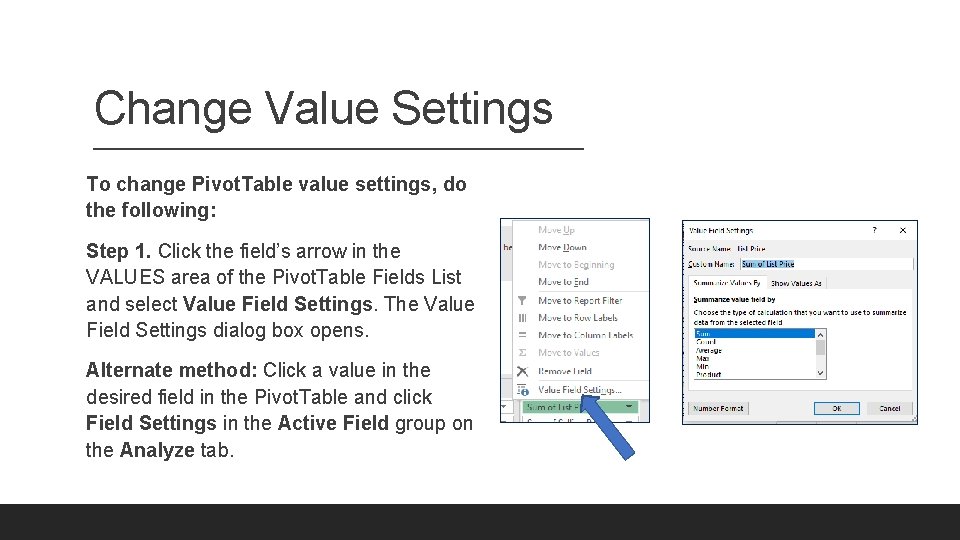
Change Value Settings To change Pivot. Table value settings, do the following: Step 1. Click the field’s arrow in the VALUES area of the Pivot. Table Fields List and select Value Field Settings. The Value Field Settings dialog box opens. Alternate method: Click a value in the desired field in the Pivot. Table and click Field Settings in the Active Field group on the Analyze tab.

Change Value Settings To change Pivot. Table value settings, do the following: Step 2. Type the name you want to appear as the column label in the Custom Name box. Step 3. Select the summary statistical function you want to use to summarize the values in the Summarize value field by list. Step 4. Click Number Format to open an abbreviated version of the Format Cells dialog box. Select a number type (e. g. , Accounting, in the Category list; select other settings as desired, and then click OK. Step 5. Click OK in the Value Field Settings dialog box.

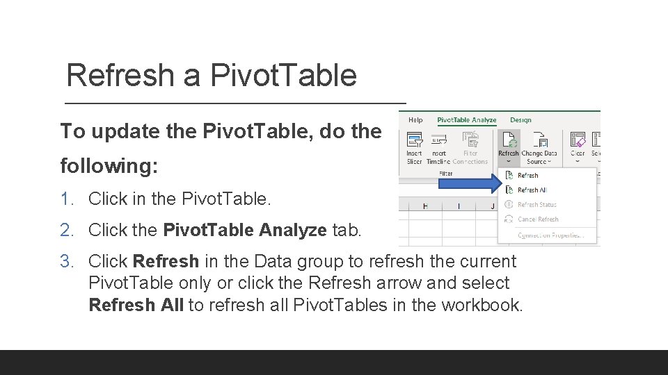
Refresh a Pivot. Table To update the Pivot. Table, do the following: 1. Click in the Pivot. Table. 2. Click the Pivot. Table Analyze tab. 3. Click Refresh in the Data group to refresh the current Pivot. Table only or click the Refresh arrow and select Refresh All to refresh all Pivot. Tables in the workbook.

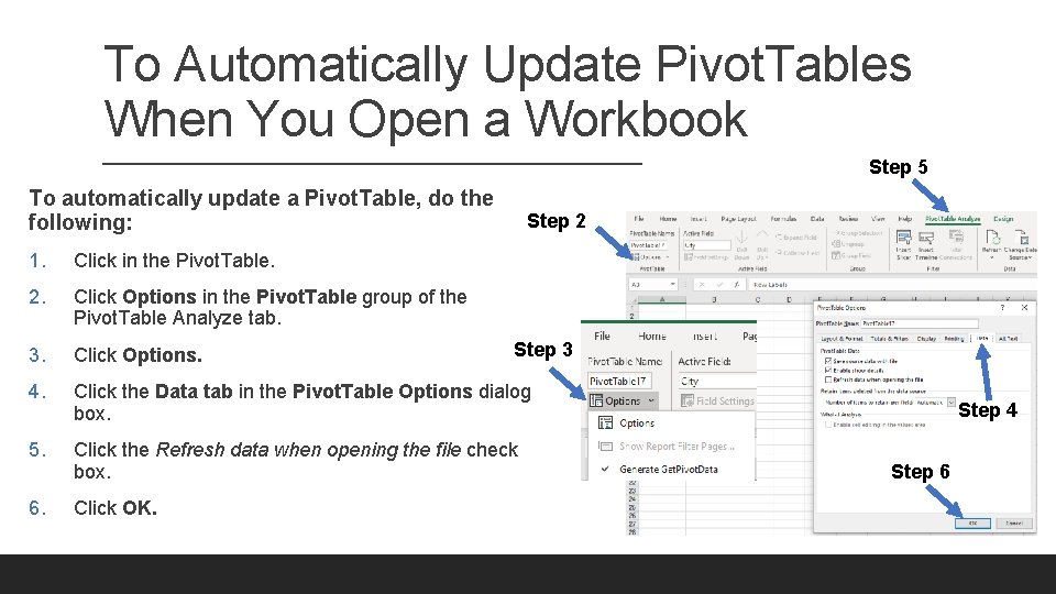
To Automatically Update Pivot. Tables When You Open a Workbook Step 5 To automatically update a Pivot. Table, do the following: Step 2 1. Click in the Pivot. Table. 2. Click Options in the Pivot. Table group of the Pivot. Table Analyze tab. 3. Click Options. 4. Click the Data tab in the Pivot. Table Options dialog box. 5. Click the Refresh data when opening the file check box. 6. Click OK. Step 3 Step 4 Step 6

Clear Pivot. Table Fields To reset a Pivot. Table back to a blank Pivot. Table, do the following: ØClick within the Pivot. Table ØClick Clear in the Actions group (Analyze tab) ØSelect Clear All.

Thank You!! Please take a minute to complete the poll. Questions? ?

Express Excel – Managing Large Worksheets Handouts, Links to Additional Resources HTTPS: //WWW. MTATERESEARCH. COM/ QUESTIONS OR COMMENTS? MARSHA@MTATERESEARCH. COM

Works Cited Frye, Curtis D. “PIVOTTABLE ANNOYANCES” in Excel Annoyances. O’Reilly, https: //www. oreilly. com/library/view/excelannoyances/0596007280/ch 04 s 04. html (accessed 27 April 2020). Microsoft. “Create a Pivot. Table to Analyze Worksheet Data. ” https: //support. office. com/en-us/article/create-a-pivottable-toanalyze-worksheet-data-a 9 a 84538 -bfe 9 -40 a 9 -a 8 e 9 -f 99134456576 (accessed 27 April 2020). Poatsy, Mary Anne, series ed. Microsoft Excel 2016 Comprehensive. Boston, Pearson, 2017.