EXCEL Editing and Formatting Worksheets Section 2 Paradigm

EXCEL Editing and Formatting Worksheets Section 2 © Paradigm Publishing Inc.

Skills Links to Activities 2. 1 2. 2 2. 3 2. 4 2. 5 2. 6 2. 7 2. 8 • Edit the content of cells • Clear cells and cell formats • Use proofing tools • Insert and delete columns and rows • Move and copy cells • Use Paste Options to link cells 2. 9 2. 10 2. 11 • Create formulas using absolute references • Adjust column width and row height • Change the font, size, style, and color of cells © Paradigm Publishing Inc.

Skills Links to Activities 2. 1 2. 2 • Apply numeric formats and adjust the number of decimal places • Use Undo, Redo, and Repeat 2. 3 2. 4 2. 5 2. 6 2. 7 2. 8 2. 9 2. 10 2. 11 • Change cell alignment and indentation • Add borders and shading • Copy formats using Format Painter • Apply cell styles • Find and replace cell entries and formats • Freeze and unfreeze panes • Change the zoom percentage © Paradigm Publishing Inc.

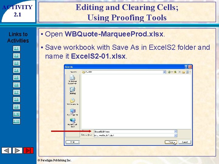
Editing and Clearing Cells; Using Proofing Tools ACTIVITY 2. 1 Links to Activities 2. 1 2. 2 • Open WBQuote-Marquee. Prod. xlsx. • Save workbook with Save As in Excel. S 2 folder and name it Excel. S 2 -01. xlsx. 2. 3 2. 4 2. 5 2. 6 2. 7 2. 8 2. 9 2. 10 2. 11 Excel. S 2 -01. xlsx © Paradigm Publishing Inc.

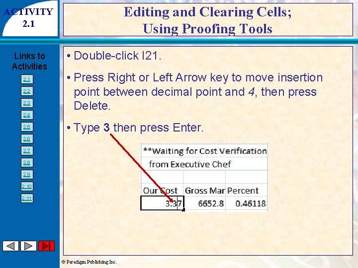
Editing and Clearing Cells; Using Proofing Tools ACTIVITY 2. 1 Links to Activities 2. 1 2. 2 2. 3 2. 4 2. 5 • Double-click I 21. • Press Right or Left Arrow key to move insertion point between decimal point and 4, then press Delete. • Type 3 then press Enter. 2. 6 2. 7 2. 8 2. 9 2. 10 2. 11 © Paradigm Publishing Inc.

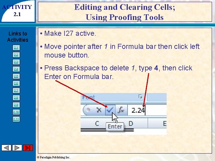
Editing and Clearing Cells; Using Proofing Tools ACTIVITY 2. 1 Links to Activities 2. 1 2. 2 • Make I 27 active. • Move pointer after 1 in Formula bar then click left mouse button. 2. 3 2. 4 2. 5 • Press Backspace to delete 1, type 4, then click Enter on Formula bar. 2. 6 2. 7 2. 8 2. 9 2. 10 2. 11 © Paradigm Publishing Inc.

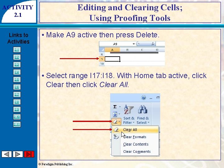
Editing and Clearing Cells; Using Proofing Tools ACTIVITY 2. 1 Links to Activities • Make A 9 active then press Delete. 2. 1 2. 2 2. 3 2. 4 2. 5 2. 6 • Select range I 17: I 18. With Home tab active, click Clear then click Clear All. 2. 7 2. 8 2. 9 2. 10 2. 11 © Paradigm Publishing Inc.

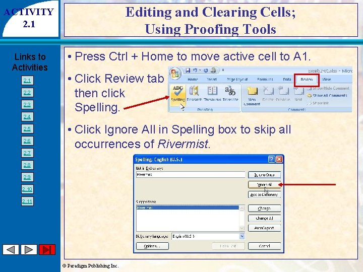
Editing and Clearing Cells; Using Proofing Tools ACTIVITY 2. 1 Links to Activities 2. 1 2. 2 2. 3 2. 4 2. 5 2. 6 2. 7 • Press Ctrl + Home to move active cell to A 1. • Click Review tab then click Spelling. • Click Ignore All in Spelling box to skip all occurrences of Rivermist. 2. 8 2. 9 2. 10 2. 11 © Paradigm Publishing Inc.

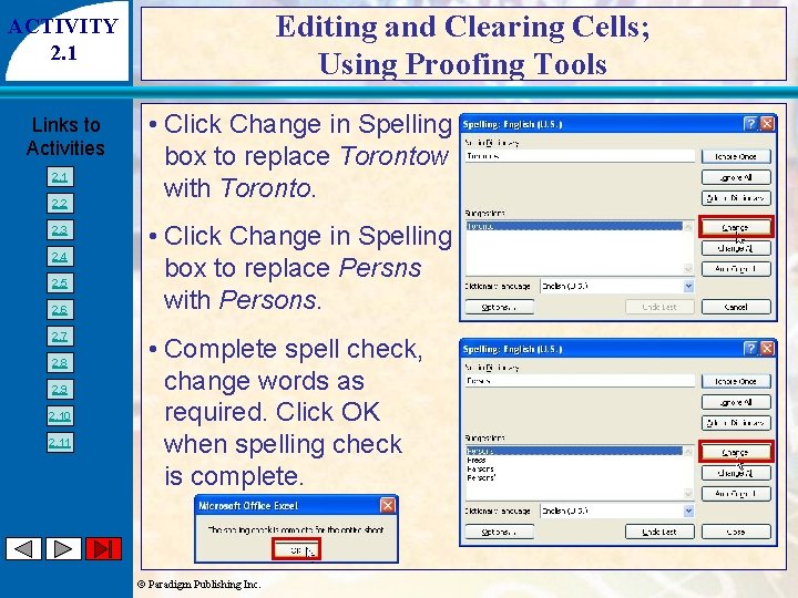
Editing and Clearing Cells; Using Proofing Tools ACTIVITY 2. 1 Links to Activities 2. 1 2. 2 2. 3 2. 4 2. 5 2. 6 2. 7 2. 8 2. 9 2. 10 2. 11 • Click Change in Spelling box to replace Torontow with Toronto. • Click Change in Spelling box to replace Persns with Persons. • Complete spell check, change words as required. Click OK when spelling check is complete. © Paradigm Publishing Inc.

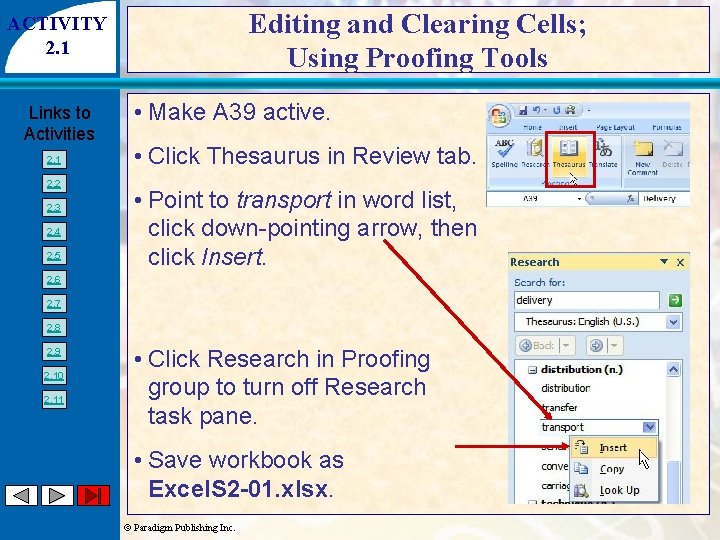
Editing and Clearing Cells; Using Proofing Tools ACTIVITY 2. 1 Links to Activities 2. 1 2. 2 2. 3 2. 4 2. 5 • Make A 39 active. • Click Thesaurus in Review tab. • Point to transport in word list, click down-pointing arrow, then click Insert. 2. 6 2. 7 2. 8 2. 9 2. 10 2. 11 • Click Research in Proofing group to turn off Research task pane. • Save workbook as Excel. S 2 -01. xlsx. © Paradigm Publishing Inc.

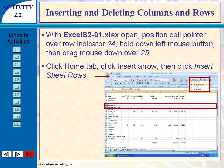
ACTIVITY 2. 2 Links to Activities 2. 1 2. 2 2. 3 2. 4 2. 5 Inserting and Deleting Columns and Rows • With Excel. S 2 -01. xlsx open, position cell pointer over row indicator 24, hold down left mouse button, then drag mouse down over 25. • Click Home tab, click Insert arrow, then click Insert Sheet Rows. 2. 6 2. 7 2. 8 2. 9 2. 10 2. 11 © Paradigm Publishing Inc.

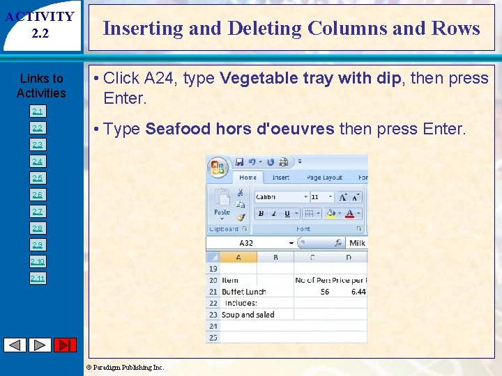
ACTIVITY 2. 2 Inserting and Deleting Columns and Rows Links to Activities • Click A 24, type Vegetable tray with dip, then press Enter. 2. 1 2. 2 • Type Seafood hors d'oeuvres then press Enter. 2. 3 2. 4 2. 5 2. 6 2. 7 2. 8 2. 9 2. 10 2. 11 © Paradigm Publishing Inc.

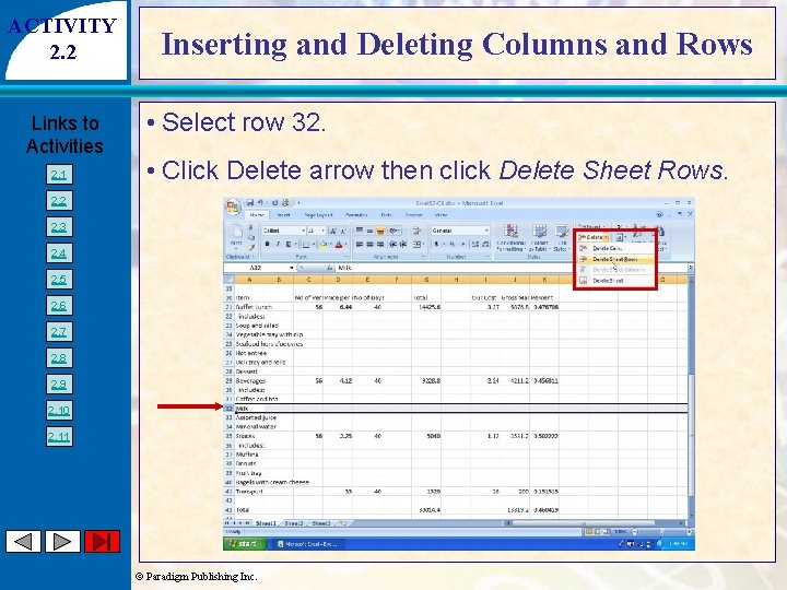
ACTIVITY 2. 2 Links to Activities 2. 1 Inserting and Deleting Columns and Rows • Select row 32. • Click Delete arrow then click Delete Sheet Rows. 2. 2 2. 3 2. 4 2. 5 2. 6 2. 7 2. 8 2. 9 2. 10 2. 11 © Paradigm Publishing Inc.

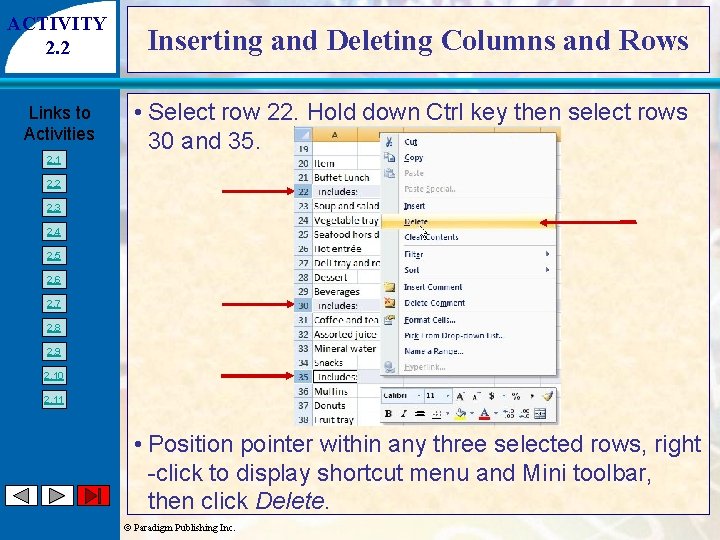
ACTIVITY 2. 2 Links to Activities 2. 1 Inserting and Deleting Columns and Rows • Select row 22. Hold down Ctrl key then select rows 30 and 35. 2. 2 2. 3 2. 4 2. 5 2. 6 2. 7 2. 8 2. 9 2. 10 2. 11 • Position pointer within any three selected rows, right -click to display shortcut menu and Mini toolbar, then click Delete. © Paradigm Publishing Inc.

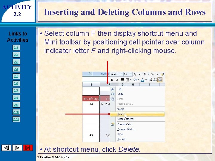
ACTIVITY 2. 2 Links to Activities 2. 1 2. 2 Inserting and Deleting Columns and Rows • Select column F then display shortcut menu and Mini toolbar by positioning cell pointer over column indicator letter F and right-clicking mouse. 2. 3 2. 4 2. 5 2. 6 2. 7 2. 8 2. 9 2. 10 2. 11 • At shortcut menu, click Delete. © Paradigm Publishing Inc.

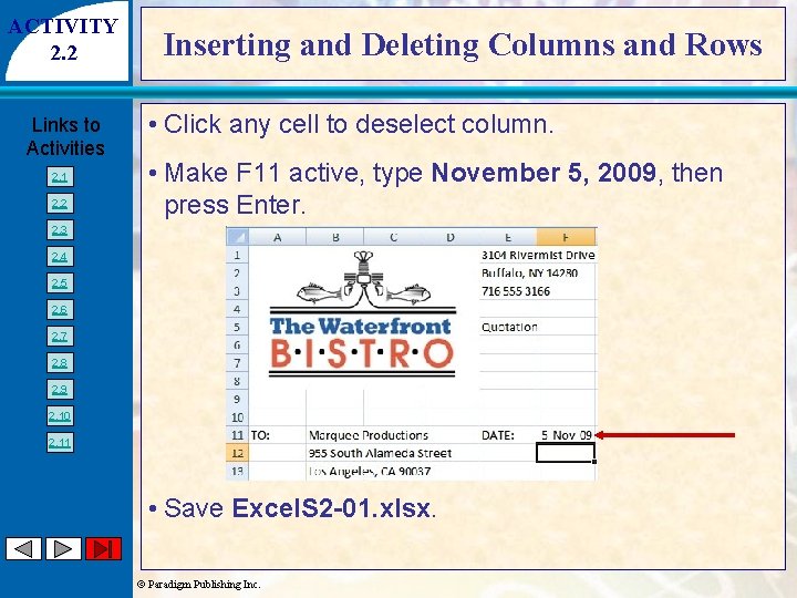
ACTIVITY 2. 2 Links to Activities 2. 1 2. 2 Inserting and Deleting Columns and Rows • Click any cell to deselect column. • Make F 11 active, type November 5, 2009, then press Enter. 2. 3 2. 4 2. 5 2. 6 2. 7 2. 8 2. 9 2. 10 2. 11 • Save Excel. S 2 -01. xlsx. © Paradigm Publishing Inc.

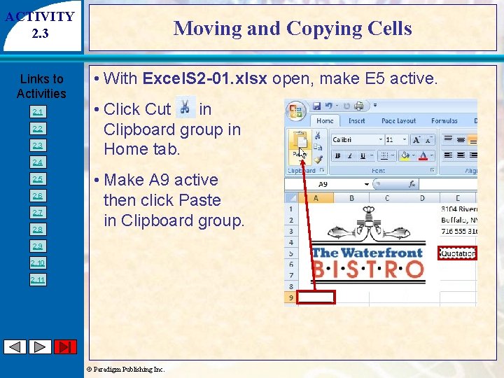
ACTIVITY 2. 3 Links to Activities 2. 1 2. 2 2. 3 2. 4 2. 5 2. 6 2. 7 2. 8 Moving and Copying Cells • With Excel. S 2 -01. xlsx open, make E 5 active. • Click Cut in Clipboard group in Home tab. • Make A 9 active then click Paste in Clipboard group. 2. 9 2. 10 2. 11 © Paradigm Publishing Inc.

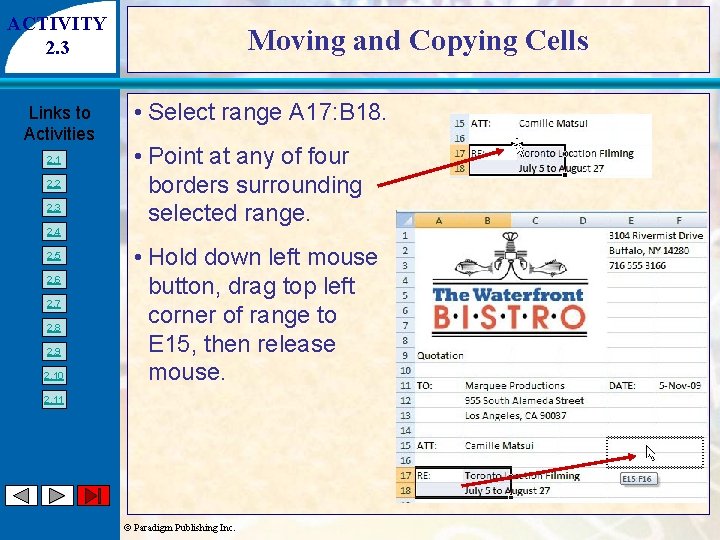
ACTIVITY 2. 3 Links to Activities 2. 1 2. 2 2. 3 2. 4 2. 5 2. 6 2. 7 2. 8 2. 9 2. 10 Moving and Copying Cells • Select range A 17: B 18. • Point at any of four borders surrounding selected range. • Hold down left mouse button, drag top left corner of range to E 15, then release mouse. 2. 11 © Paradigm Publishing Inc.

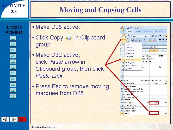
ACTIVITY 2. 3 Links to Activities 2. 1 2. 2 Moving and Copying Cells • Make D 28 active. • Click Copy group. in Clipboard 2. 3 2. 4 2. 5 2. 6 2. 7 2. 8 2. 9 2. 10 2. 11 • Make D 32 active, click Paste arrow in Clipboard group, then click Paste Link. • Press Esc to remove moving marquee from D 28. © Paradigm Publishing Inc.

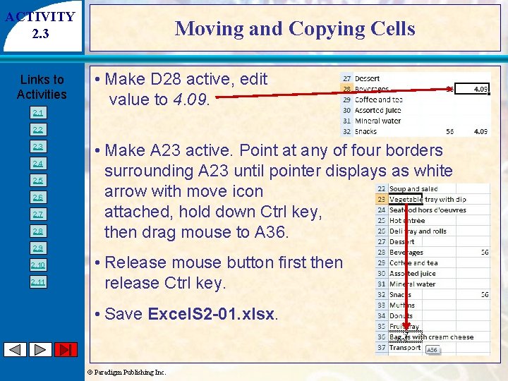
ACTIVITY 2. 3 Links to Activities 2. 1 Moving and Copying Cells • Make D 28 active, edit value to 4. 09. 2. 2 2. 3 2. 4 2. 5 2. 6 2. 7 2. 8 • Make A 23 active. Point at any of four borders surrounding A 23 until pointer displays as white arrow with move icon attached, hold down Ctrl key, then drag mouse to A 36. 2. 9 2. 10 2. 11 • Release mouse button first then release Ctrl key. • Save Excel. S 2 -01. xlsx. © Paradigm Publishing Inc.

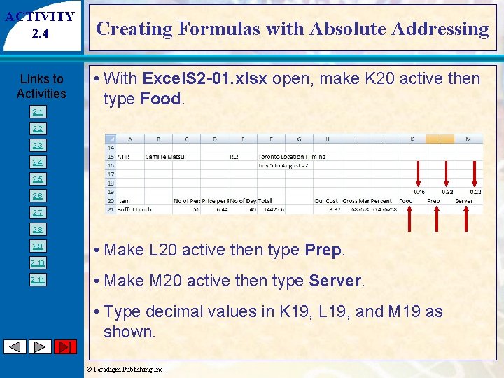
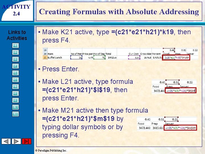
ACTIVITY 2. 4 Links to Activities 2. 1 Creating Formulas with Absolute Addressing • With Excel. S 2 -01. xlsx open, make K 20 active then type Food. 2. 2 2. 3 2. 4 2. 5 2. 6 2. 7 2. 8 2. 9 2. 10 2. 11 • Make L 20 active then type Prep. • Make M 20 active then type Server. • Type decimal values in K 19, L 19, and M 19 as shown. © Paradigm Publishing Inc.

ACTIVITY 2. 4 Links to Activities 2. 1 Creating Formulas with Absolute Addressing • Make K 21 active, type =(c 21*e 21*h 21)*k 19, then press F 4. 2. 2 2. 3 2. 4 2. 5 2. 6 2. 7 2. 8 2. 9 2. 10 2. 11 • Press Enter. • Make L 21 active, type formula =(c 21*e 21*h 21)*$I$19, then press Enter. • Make M 21 active then type formula =(c 21*e 21*h 21)*$m$19 by typing dollar symbols or by pressing F 4. © Paradigm Publishing Inc.

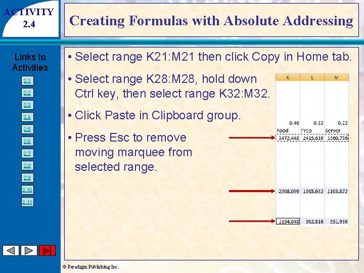
ACTIVITY 2. 4 Links to Activities 2. 1 2. 2 Creating Formulas with Absolute Addressing • Select range K 21: M 21 then click Copy in Home tab. • Select range K 28: M 28, hold down Ctrl key, then select range K 32: M 32. 2. 3 2. 4 2. 5 2. 6 2. 7 2. 8 • Click Paste in Clipboard group. • Press Esc to remove moving marquee from selected range. 2. 9 2. 10 2. 11 © Paradigm Publishing Inc.

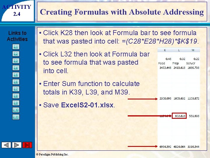
ACTIVITY 2. 4 Links to Activities 2. 1 2. 2 2. 3 2. 4 2. 5 2. 6 2. 7 2. 8 2. 9 2. 10 Creating Formulas with Absolute Addressing • Click K 28 then look at Formula bar to see formula that was pasted into cell: =(C 28*E 28*H 28)*$K$19. • Click L 32 then look at Formula bar to see formula that was pasted into cell. • Enter Sum function to calculate totals in K 39, L 39, and M 39. • Save Excel. S 2 -01. xlsx. 2. 11 © Paradigm Publishing Inc.

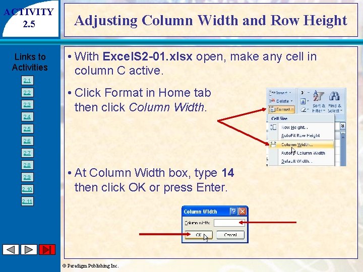
ACTIVITY 2. 5 Links to Activities Adjusting Column Width and Row Height • With Excel. S 2 -01. xlsx open, make any cell in column C active. 2. 1 2. 2 2. 3 2. 4 • Click Format in Home tab then click Column Width. 2. 5 2. 6 2. 7 2. 8 2. 9 2. 10 • At Column Width box, type 14 then click OK or press Enter. 2. 11 © Paradigm Publishing Inc.

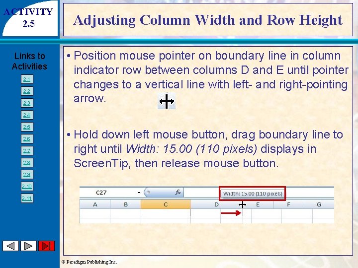
ACTIVITY 2. 5 Links to Activities 2. 1 2. 2 2. 3 Adjusting Column Width and Row Height • Position mouse pointer on boundary line in column indicator row between columns D and E until pointer changes to a vertical line with left- and right-pointing arrow. 2. 4 2. 5 2. 6 2. 7 2. 8 • Hold down left mouse button, drag boundary line to right until Width: 15. 00 (110 pixels) displays in Screen. Tip, then release mouse button. 2. 9 2. 10 2. 11 © Paradigm Publishing Inc.

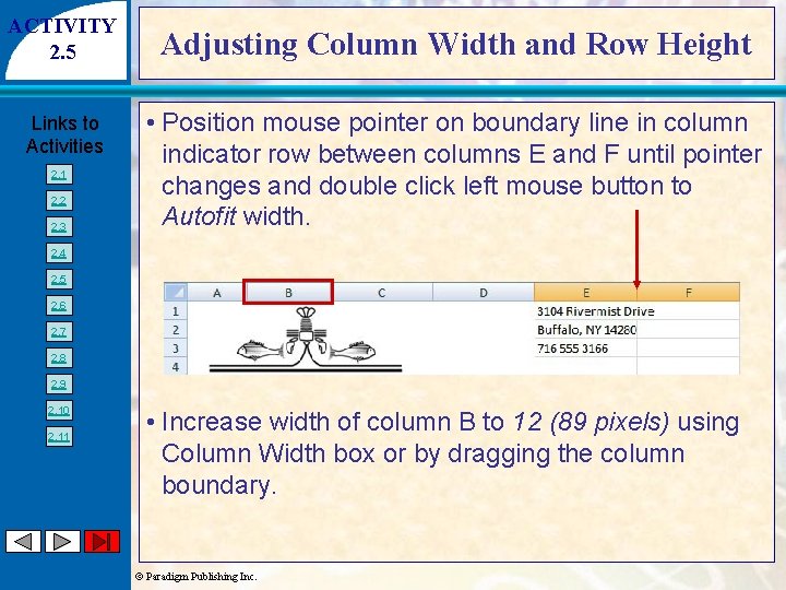
ACTIVITY 2. 5 Links to Activities 2. 1 2. 2 2. 3 Adjusting Column Width and Row Height • Position mouse pointer on boundary line in column indicator row between columns E and F until pointer changes and double click left mouse button to Autofit width. 2. 4 2. 5 2. 6 2. 7 2. 8 2. 9 2. 10 2. 11 • Increase width of column B to 12 (89 pixels) using Column Width box or by dragging the column boundary. © Paradigm Publishing Inc.

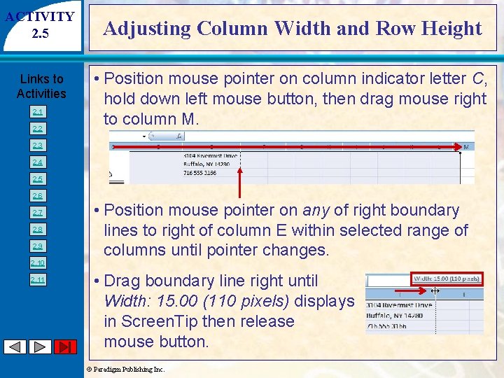
ACTIVITY 2. 5 Links to Activities 2. 1 2. 2 Adjusting Column Width and Row Height • Position mouse pointer on column indicator letter C, hold down left mouse button, then drag mouse right to column M. 2. 3 2. 4 2. 5 2. 6 2. 7 2. 8 2. 9 2. 10 2. 11 • Position mouse pointer on any of right boundary lines to right of column E within selected range of columns until pointer changes. • Drag boundary line right until Width: 15. 00 (110 pixels) displays in Screen. Tip then release mouse button. © Paradigm Publishing Inc.

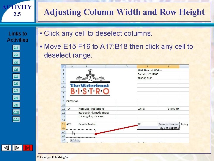
ACTIVITY 2. 5 Links to Activities 2. 1 2. 2 Adjusting Column Width and Row Height • Click any cell to deselect columns. • Move E 15: F 16 to A 17: B 18 then click any cell to deselect range. 2. 3 2. 4 2. 5 2. 6 2. 7 2. 8 2. 9 2. 10 2. 11 © Paradigm Publishing Inc.

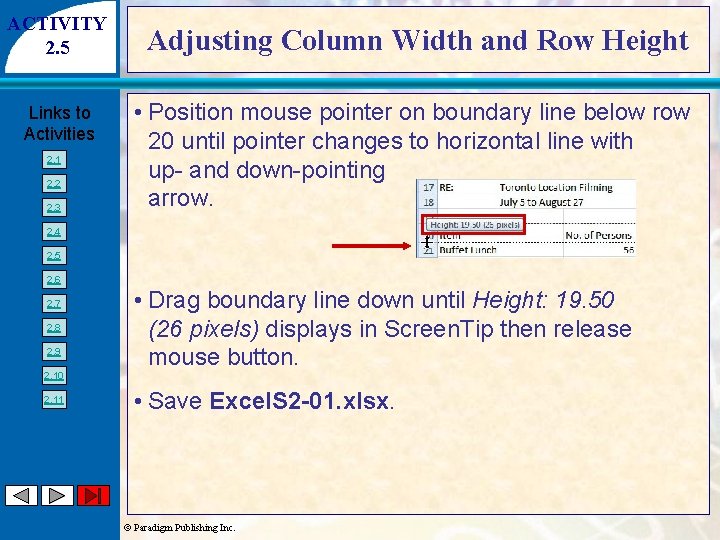
ACTIVITY 2. 5 Links to Activities 2. 1 2. 2 2. 3 Adjusting Column Width and Row Height • Position mouse pointer on boundary line below row 20 until pointer changes to horizontal line with up- and down-pointing arrow. 2. 4 2. 5 2. 6 2. 7 2. 8 2. 9 2. 10 2. 11 • Drag boundary line down until Height: 19. 50 (26 pixels) displays in Screen. Tip then release mouse button. • Save Excel. S 2 -01. xlsx. © Paradigm Publishing Inc.

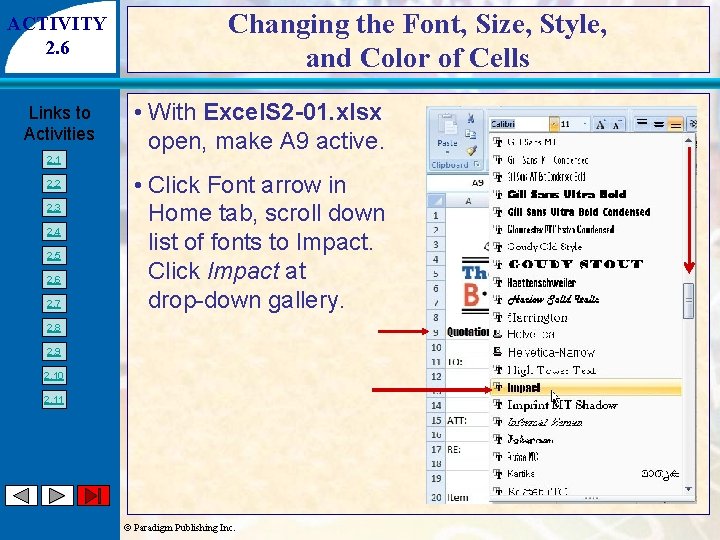
ACTIVITY 2. 6 Links to Activities 2. 1 2. 2 2. 3 2. 4 2. 5 2. 6 2. 7 Changing the Font, Size, Style, and Color of Cells • With Excel. S 2 -01. xlsx open, make A 9 active. • Click Font arrow in Home tab, scroll down list of fonts to Impact. Click Impact at drop-down gallery. 2. 8 2. 9 2. 10 2. 11 © Paradigm Publishing Inc.

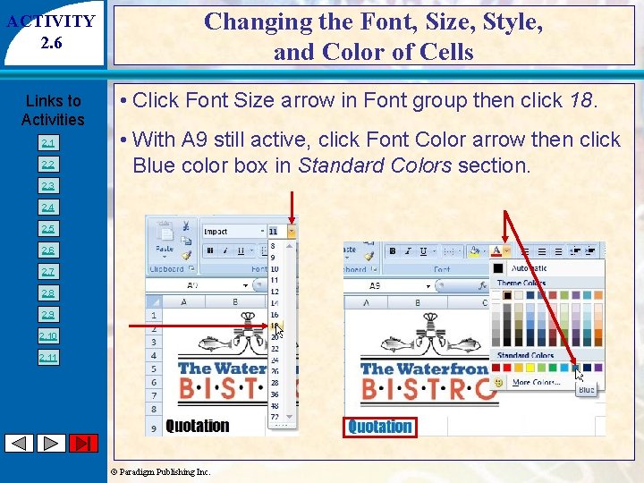
ACTIVITY 2. 6 Links to Activities 2. 1 2. 2 Changing the Font, Size, Style, and Color of Cells • Click Font Size arrow in Font group then click 18. • With A 9 still active, click Font Color arrow then click Blue color box in Standard Colors section. 2. 3 2. 4 2. 5 2. 6 2. 7 2. 8 2. 9 2. 10 2. 11 © Paradigm Publishing Inc.

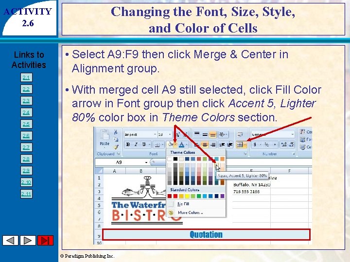
ACTIVITY 2. 6 Links to Activities 2. 1 2. 2 2. 3 2. 4 2. 5 Changing the Font, Size, Style, and Color of Cells • Select A 9: F 9 then click Merge & Center in Alignment group. • With merged cell A 9 still selected, click Fill Color arrow in Font group then click Accent 5, Lighter 80% color box in Theme Colors section. 2. 6 2. 7 2. 8 2. 9 2. 10 2. 11 © Paradigm Publishing Inc.

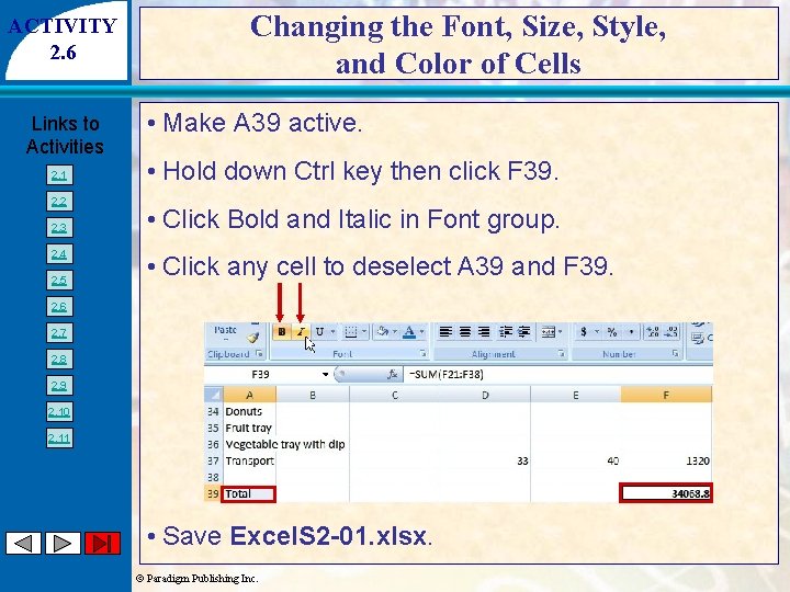
ACTIVITY 2. 6 Links to Activities 2. 1 2. 2 2. 3 2. 4 2. 5 Changing the Font, Size, Style, and Color of Cells • Make A 39 active. • Hold down Ctrl key then click F 39. • Click Bold and Italic in Font group. • Click any cell to deselect A 39 and F 39. 2. 6 2. 7 2. 8 2. 9 2. 10 2. 11 • Save Excel. S 2 -01. xlsx. © Paradigm Publishing Inc.

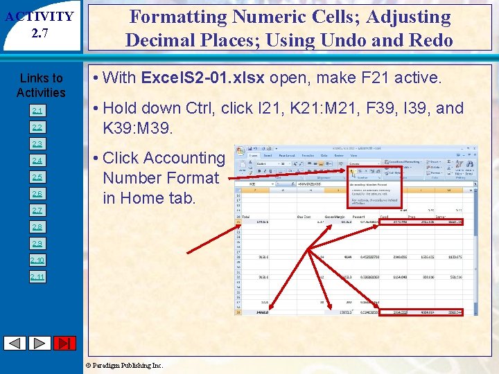
ACTIVITY 2. 7 Links to Activities 2. 1 2. 2 Formatting Numeric Cells; Adjusting Decimal Places; Using Undo and Redo • With Excel. S 2 -01. xlsx open, make F 21 active. • Hold down Ctrl, click I 21, K 21: M 21, F 39, I 39, and K 39: M 39. 2. 3 2. 4 2. 5 2. 6 2. 7 • Click Accounting Number Format in Home tab. 2. 8 2. 9 2. 10 2. 11 © Paradigm Publishing Inc.

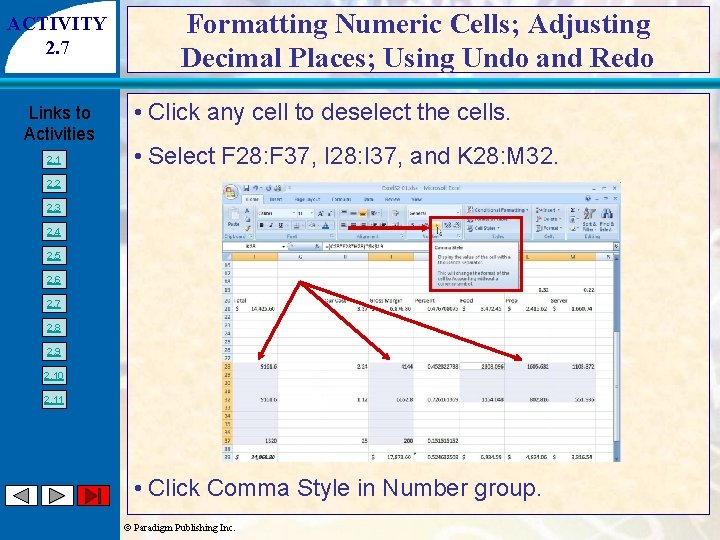
ACTIVITY 2. 7 Links to Activities 2. 1 Formatting Numeric Cells; Adjusting Decimal Places; Using Undo and Redo • Click any cell to deselect the cells. • Select F 28: F 37, I 28: I 37, and K 28: M 32. 2. 2 2. 3 2. 4 2. 5 2. 6 2. 7 2. 8 2. 9 2. 10 2. 11 • Click Comma Style in Number group. © Paradigm Publishing Inc.

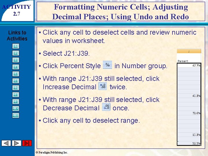
ACTIVITY 2. 7 Links to Activities 2. 1 2. 2 Formatting Numeric Cells; Adjusting Decimal Places; Using Undo and Redo • Click any cell to deselect cells and review numeric values in worksheet. • Select J 21: J 39. 2. 3 2. 4 2. 5 2. 6 2. 7 2. 8 2. 9 2. 10 2. 11 • Click Percent Style in Number group. • With range J 21: J 39 still selected, click Increase Decimal twice. • With range J 21: J 39 still selected, click Decrease Decimal once. • Click any cell to deselect range. © Paradigm Publishing Inc.

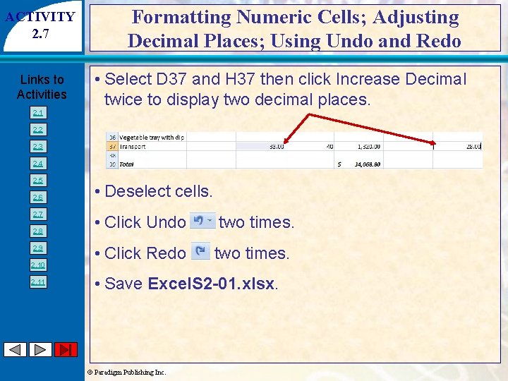
ACTIVITY 2. 7 Links to Activities 2. 1 Formatting Numeric Cells; Adjusting Decimal Places; Using Undo and Redo • Select D 37 and H 37 then click Increase Decimal twice to display two decimal places. 2. 2 2. 3 2. 4 2. 5 2. 6 2. 7 2. 8 2. 9 2. 10 2. 11 • Deselect cells. • Click Undo two times. • Click Redo two times. • Save Excel. S 2 -01. xlsx. © Paradigm Publishing Inc.

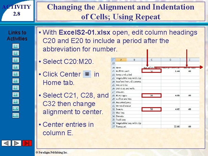
ACTIVITY 2. 8 Links to Activities 2. 1 2. 2 2. 3 2. 4 2. 5 2. 6 2. 7 2. 8 2. 9 2. 10 2. 11 Changing the Alignment and Indentation of Cells; Using Repeat • With Excel. S 2 -01. xlsx open, edit column headings C 20 and E 20 to include a period after the abbreviation for number. • Select C 20: M 20. • Click Center Home tab. in • Select C 21, C 28, and C 32 then change alignment to center. • Center entries in column E. © Paradigm Publishing Inc.

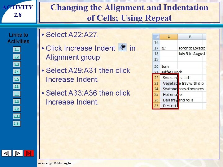
ACTIVITY 2. 8 Links to Activities 2. 1 2. 2 Changing the Alignment and Indentation of Cells; Using Repeat • Select A 22: A 27. • Click Increase Indent Alignment group. in 2. 3 2. 4 2. 5 • Select A 29: A 31 then click Increase Indent. 2. 6 2. 7 2. 8 • Select A 33: A 36 then click Increase Indent. 2. 9 2. 10 2. 11 © Paradigm Publishing Inc.

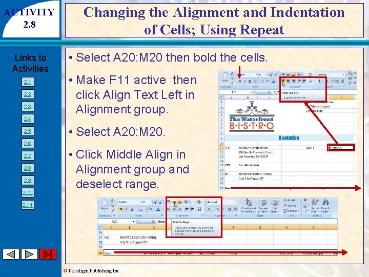
ACTIVITY 2. 8 Links to Activities 2. 1 2. 2 2. 3 2. 4 2. 5 Changing the Alignment and Indentation of Cells; Using Repeat • Select A 20: M 20 then bold the cells. • Make F 11 active then click Align Text Left in Alignment group. • Select A 20: M 20. 2. 6 2. 7 2. 8 2. 9 2. 10 • Click Middle Align in Alignment group and deselect range. 2. 11 © Paradigm Publishing Inc.

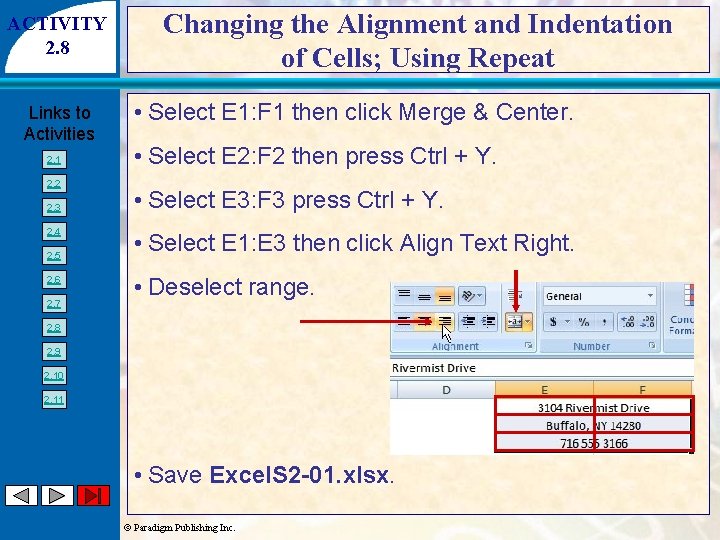
ACTIVITY 2. 8 Links to Activities 2. 1 2. 2 2. 3 2. 4 2. 5 2. 6 2. 7 Changing the Alignment and Indentation of Cells; Using Repeat • Select E 1: F 1 then click Merge & Center. • Select E 2: F 2 then press Ctrl + Y. • Select E 3: F 3 press Ctrl + Y. • Select E 1: E 3 then click Align Text Right. • Deselect range. 2. 8 2. 9 2. 10 2. 11 • Save Excel. S 2 -01. xlsx. © Paradigm Publishing Inc.

ACTIVITY 2. 9 Links to Activities 2. 1 2. 2 Adding Borders and Shading; Copying Formats with Format Painter; Using Cell Styles • With Excel. S 2 -01. xlsx open, change width of column A to 11. 00 (82 pixels). • Auto. Fit columns C–F, and H–M. 2. 3 2. 4 • Change width of column G to 4. 00 (33 pixels). 2. 5 2. 6 2. 7 2. 8 2. 9 2. 10 2. 11 © Paradigm Publishing Inc.

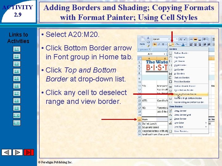
ACTIVITY 2. 9 Links to Activities 2. 1 2. 2 Adding Borders and Shading; Copying Formats with Format Painter; Using Cell Styles • Select A 20: M 20. • Click Bottom Border arrow in Font group in Home tab. 2. 3 2. 4 2. 5 • Click Top and Bottom Border at drop-down list. 2. 6 2. 7 2. 8 • Click any cell to deselect range and view border. 2. 9 2. 10 2. 11 © Paradigm Publishing Inc.

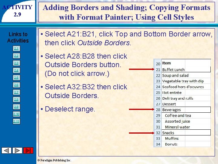
ACTIVITY 2. 9 Adding Borders and Shading; Copying Formats with Format Painter; Using Cell Styles Links to Activities • Select A 21: B 21, click Top and Bottom Border arrow, then click Outside Borders. 2. 1 2. 2 2. 3 2. 4 2. 5 2. 6 2. 7 2. 8 2. 9 2. 10 • Select A 28: B 28 then click Outside Borders button. (Do not click arrow. ) • Select A 32: B 32 then click Outside Borders. • Deselect range. 2. 11 © Paradigm Publishing Inc.

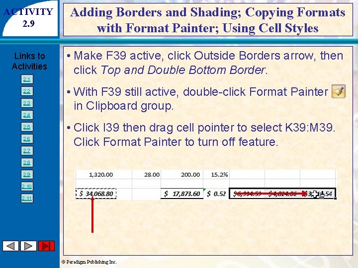
ACTIVITY 2. 9 Links to Activities 2. 1 2. 2 2. 3 2. 4 2. 5 2. 6 2. 7 Adding Borders and Shading; Copying Formats with Format Painter; Using Cell Styles • Make F 39 active, click Outside Borders arrow, then click Top and Double Bottom Border. • With F 39 still active, double-click Format Painter in Clipboard group. • Click I 39 then drag cell pointer to select K 39: M 39. Click Format Painter to turn off feature. 2. 8 2. 9 2. 10 2. 11 © Paradigm Publishing Inc.

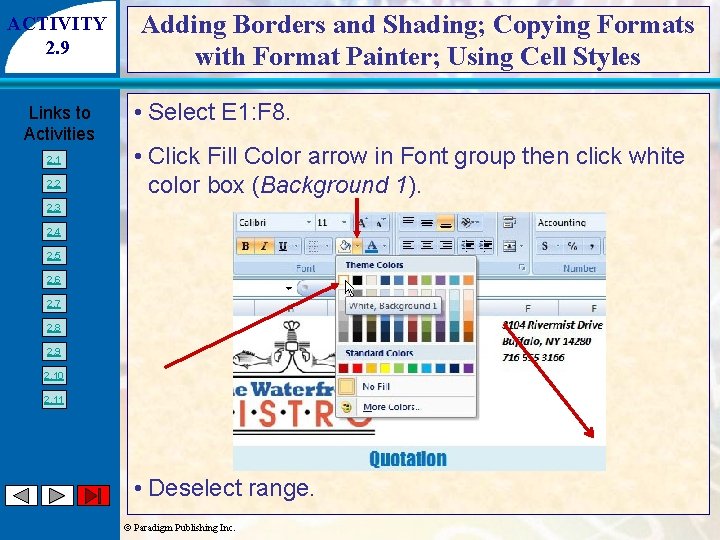
ACTIVITY 2. 9 Links to Activities 2. 1 2. 2 Adding Borders and Shading; Copying Formats with Format Painter; Using Cell Styles • Select E 1: F 8. • Click Fill Color arrow in Font group then click white color box (Background 1). 2. 3 2. 4 2. 5 2. 6 2. 7 2. 8 2. 9 2. 10 2. 11 • Deselect range. © Paradigm Publishing Inc.

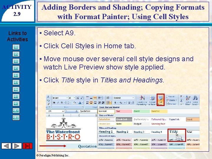
ACTIVITY 2. 9 Links to Activities 2. 1 2. 2 2. 3 2. 4 2. 5 2. 6 Adding Borders and Shading; Copying Formats with Format Painter; Using Cell Styles • Select A 9. • Click Cell Styles in Home tab. • Move mouse over several cell style designs and watch Live Preview show style applied. • Click Title style in Titles and Headings. 2. 7 2. 8 2. 9 2. 10 2. 11 © Paradigm Publishing Inc.

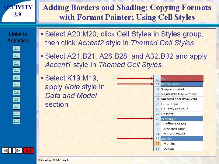
ACTIVITY 2. 9 Links to Activities 2. 1 2. 2 2. 3 2. 4 2. 5 2. 6 2. 7 2. 8 2. 9 Adding Borders and Shading; Copying Formats with Format Painter; Using Cell Styles • Select A 20: M 20, click Cell Styles in Styles group, then click Accent 2 style in Themed Cell Styles. • Select A 21: B 21, A 28: B 28, and A 32: B 32 and apply Accent 1 style in Themed Cell Styles. • Select K 19: M 19, apply Note style in Data and Model section. 2. 10 2. 11 © Paradigm Publishing Inc.

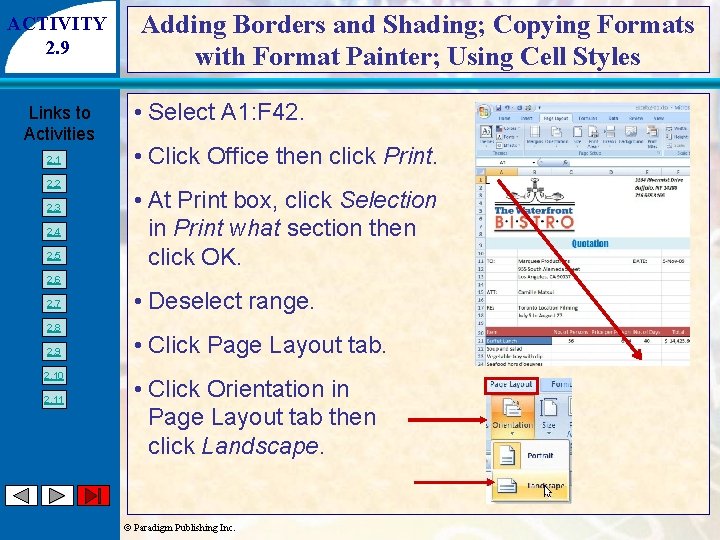
ACTIVITY 2. 9 Links to Activities 2. 1 2. 2 2. 3 2. 4 2. 5 Adding Borders and Shading; Copying Formats with Format Painter; Using Cell Styles • Select A 1: F 42. • Click Office then click Print. • At Print box, click Selection in Print what section then click OK. 2. 6 2. 7 2. 8 2. 9 2. 10 2. 11 • Deselect range. • Click Page Layout tab. • Click Orientation in Page Layout tab then click Landscape. © Paradigm Publishing Inc.

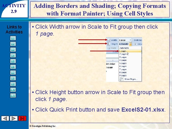
ACTIVITY 2. 9 Links to Activities 2. 1 Adding Borders and Shading; Copying Formats with Format Painter; Using Cell Styles • Click Width arrow in Scale to Fit group then click 1 page. 2. 2 2. 3 2. 4 2. 5 2. 6 2. 7 2. 8 2. 9 2. 10 2. 11 • Click Height button arrow in Scale to Fit group then click 1 page. • Click Quick Print button and save Excel. S 2 -01. xlsx. © Paradigm Publishing Inc.

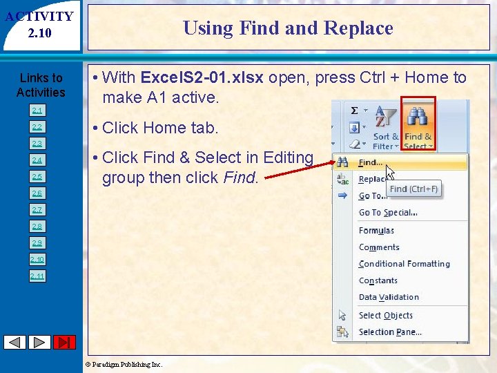
ACTIVITY 2. 10 Links to Activities 2. 1 2. 2 Using Find and Replace • With Excel. S 2 -01. xlsx open, press Ctrl + Home to make A 1 active. • Click Home tab. 2. 3 2. 4 2. 5 • Click Find & Select in Editing group then click Find. 2. 6 2. 7 2. 8 2. 9 2. 10 2. 11 © Paradigm Publishing Inc.

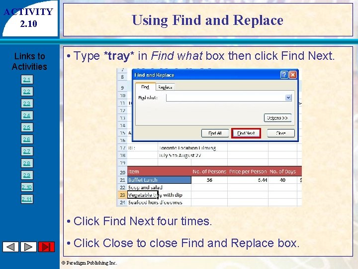
ACTIVITY 2. 10 Links to Activities Using Find and Replace • Type *tray* in Find what box then click Find Next. 2. 1 2. 2 2. 3 2. 4 2. 5 2. 6 2. 7 2. 8 2. 9 2. 10 2. 11 • Click Find Next four times. • Click Close to close Find and Replace box. © Paradigm Publishing Inc.

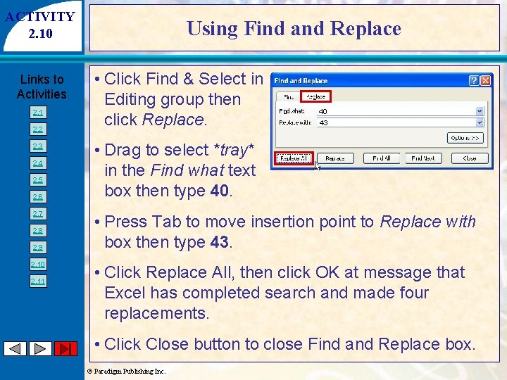
ACTIVITY 2. 10 Links to Activities 2. 1 2. 2 2. 3 2. 4 2. 5 2. 6 2. 7 2. 8 2. 9 2. 10 2. 11 Using Find and Replace • Click Find & Select in Editing group then click Replace. 40 43 • Drag to select *tray* in the Find what text box then type 40. • Press Tab to move insertion point to Replace with box then type 43. • Click Replace All, then click OK at message that Excel has completed search and made four replacements. • Click Close button to close Find and Replace box. © Paradigm Publishing Inc.

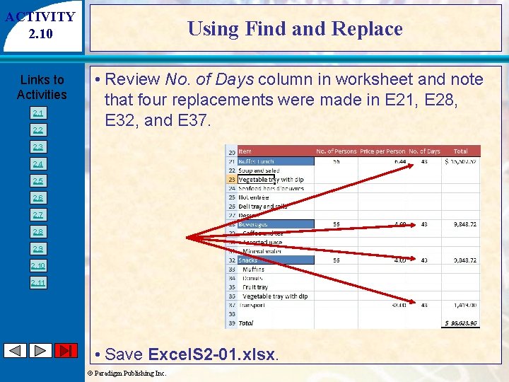
ACTIVITY 2. 10 Links to Activities 2. 1 2. 2 Using Find and Replace • Review No. of Days column in worksheet and note that four replacements were made in E 21, E 28, E 32, and E 37. 2. 3 2. 4 2. 5 2. 6 2. 7 2. 8 2. 9 2. 10 2. 11 • Save Excel. S 2 -01. xlsx. © Paradigm Publishing Inc.

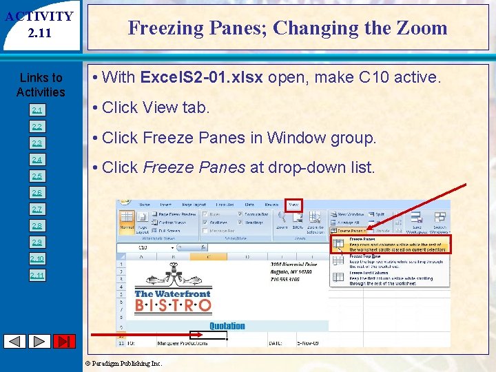
ACTIVITY 2. 11 Links to Activities 2. 1 2. 2 2. 3 2. 4 2. 5 Freezing Panes; Changing the Zoom • With Excel. S 2 -01. xlsx open, make C 10 active. • Click View tab. • Click Freeze Panes in Window group. • Click Freeze Panes at drop-down list. 2. 6 2. 7 2. 8 2. 9 2. 10 2. 11 © Paradigm Publishing Inc.

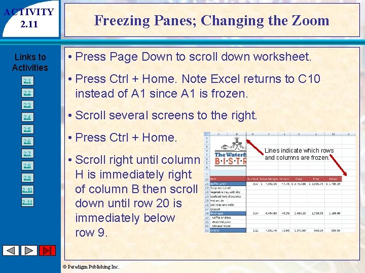
ACTIVITY 2. 11 Links to Activities 2. 1 2. 2 Freezing Panes; Changing the Zoom • Press Page Down to scroll down worksheet. • Press Ctrl + Home. Note Excel returns to C 10 instead of A 1 since A 1 is frozen. 2. 3 2. 4 2. 5 2. 6 2. 7 2. 8 2. 9 2. 10 2. 11 • Scroll several screens to the right. • Press Ctrl + Home. • Scroll right until column H is immediately right of column B then scroll down until row 20 is immediately below row 9. © Paradigm Publishing Inc. Lines indicate which rows and columns are frozen.

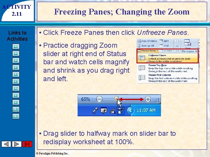
ACTIVITY 2. 11 Links to Activities 2. 1 2. 2 2. 3 2. 4 2. 5 2. 6 Freezing Panes; Changing the Zoom • Click Freeze Panes then click Unfreeze Panes. • Practice dragging Zoom slider at right end of Status bar and watch cells magnify and shrink as you drag right and left. 2. 7 2. 8 2. 9 2. 10 2. 11 • Drag slider to halfway mark on slider bar to redisplay worksheet at 100%. © Paradigm Publishing Inc.

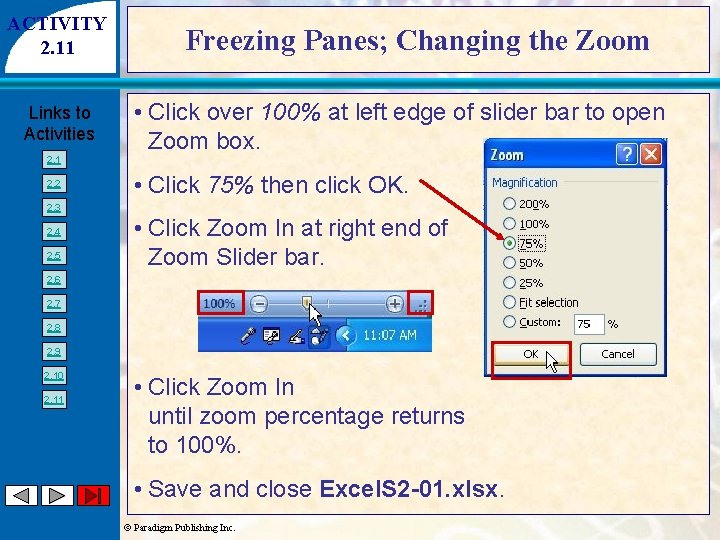
ACTIVITY 2. 11 Links to Activities 2. 1 2. 2 Freezing Panes; Changing the Zoom • Click over 100% at left edge of slider bar to open Zoom box. • Click 75% then click OK. 2. 3 2. 4 2. 5 • Click Zoom In at right end of Zoom Slider bar. 2. 6 2. 7 2. 8 2. 9 2. 10 2. 11 • Click Zoom In until zoom percentage returns to 100%. • Save and close Excel. S 2 -01. xlsx. © Paradigm Publishing Inc.