Excel Advanced Microsoft Office 2003 1 Common Functions

Excel: Advanced Microsoft Office 2003 1

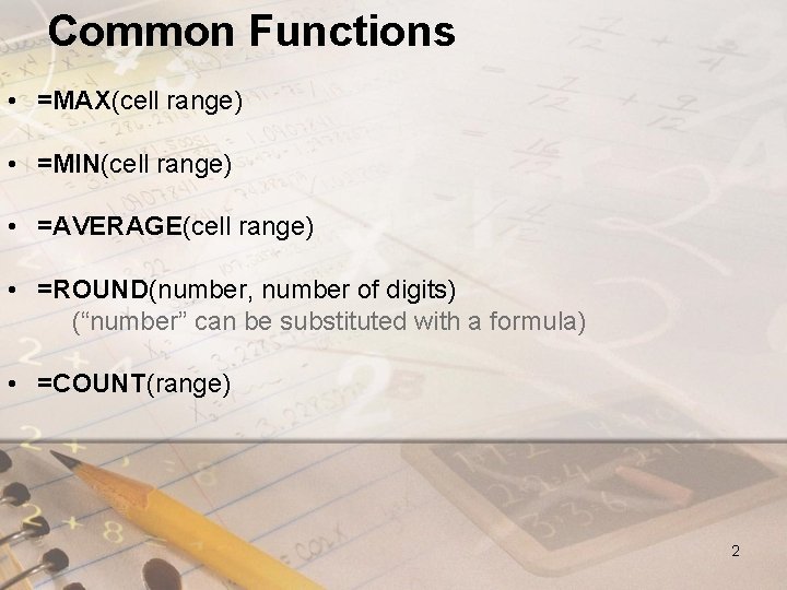
Common Functions • =MAX(cell range) • =MIN(cell range) • =AVERAGE(cell range) • =ROUND(number, number of digits) (“number” can be substituted with a formula) • =COUNT(range) 2

Conditional Functions =COUNTIF(range, criteria) =IF(Logical test, Value_if_true, Value_if_false) 3

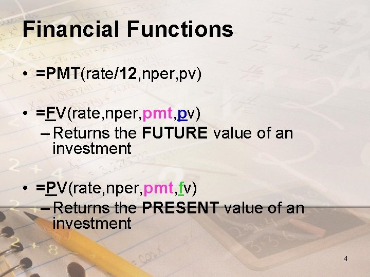
Financial Functions • =PMT(rate/12, nper, pv) • =FV(rate, nper, pmt, pv) – Returns the FUTURE value of an investment • =PV(rate, nper, pmt, fv) – Returns the PRESENT value of an investment 4

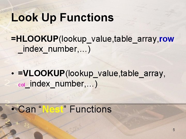
Look Up Functions =HLOOKUP(lookup_value, table_array, row _index_number, …) • =VLOOKUP(lookup_value, table_array, col_index_number, …) • Can “Nest” Functions 5

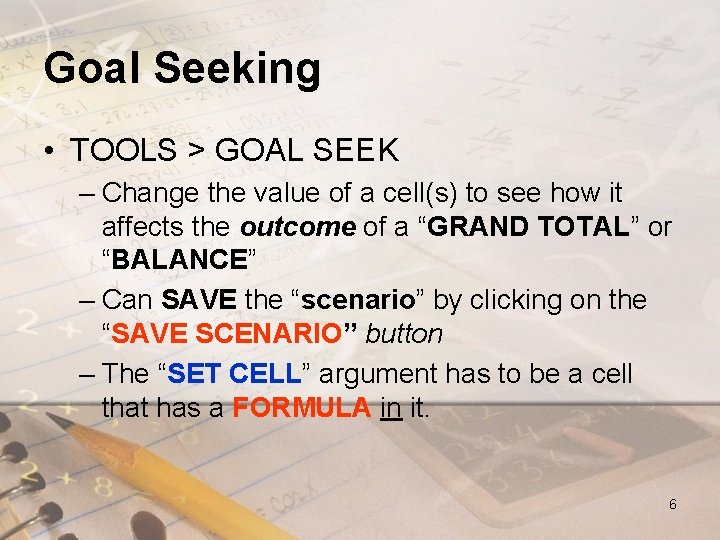
Goal Seeking • TOOLS > GOAL SEEK – Change the value of a cell(s) to see how it affects the outcome of a “GRAND TOTAL” or “BALANCE” – Can SAVE the “scenario” by clicking on the “SAVE SCENARIO” button – The “SET CELL” argument has to be a cell that has a FORMULA in it. 6

Charts • Valuable aids to compare or summarize numerical data • Many different types • Create with the charts wizard • Edit charts with a right click on the chart 7

PIVOT CHARTS • When you create a “regular” chart: – You create 1 chart for each “view” of the data that you want to see • When you create a “PIVOT” chart: – You also create a single chart BUT: • You can view the data in different ways by changing the report : – Layout OR – The detail displayed 8

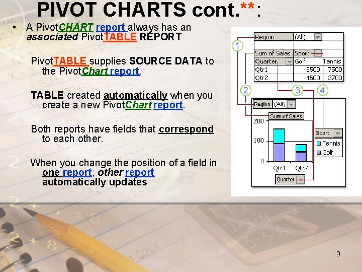
PIVOT CHARTS cont. **: • A Pivot. CHART report always has an associated Pivot. TABLE REPORT Pivot. TABLE supplies SOURCE DATA to the Pivot. Chart report. TABLE created automatically when you create a new Pivot. Chart report. Both reports have fields that correspond to each other. When you change the position of a field in one report, other report automatically updates 9

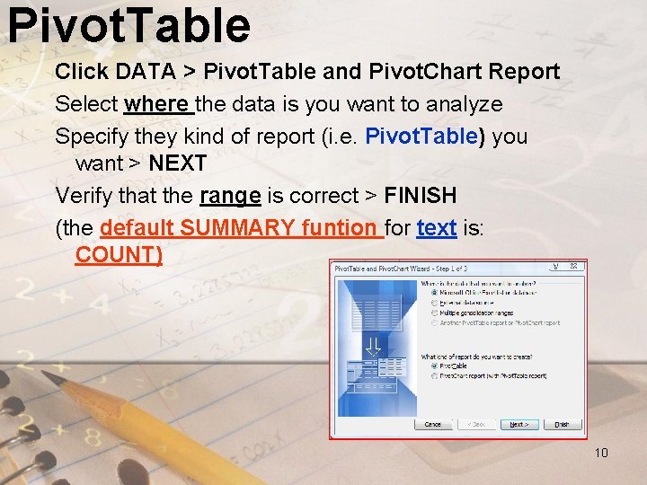
Pivot. Table Click DATA > Pivot. Table and Pivot. Chart Report Select where the data is you want to analyze Specify they kind of report (i. e. Pivot. Table) you want > NEXT Verify that the range is correct > FINISH (the default SUMMARY funtion for text is: COUNT) 10

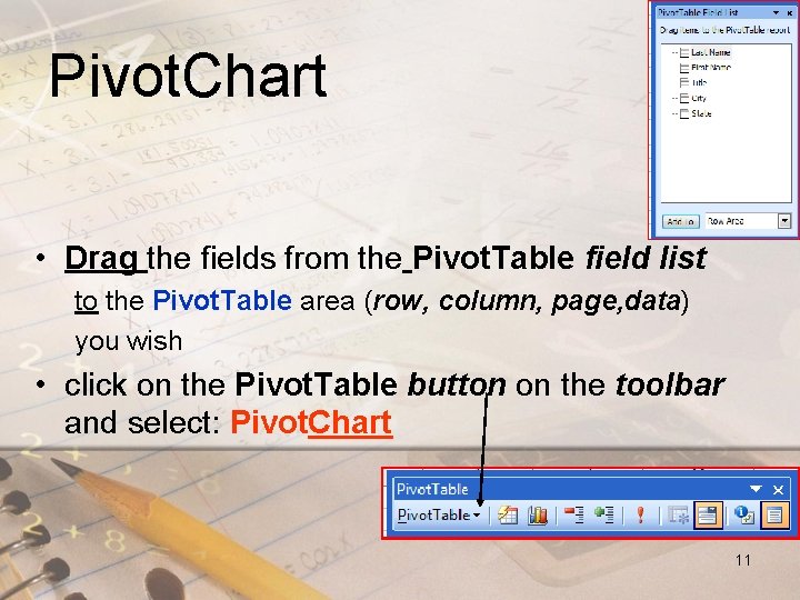
Pivot. Chart • Drag the fields from the Pivot. Table field list to the Pivot. Table area (row, column, page, data) you wish • click on the Pivot. Table button on the toolbar and select: Pivot. Chart 11

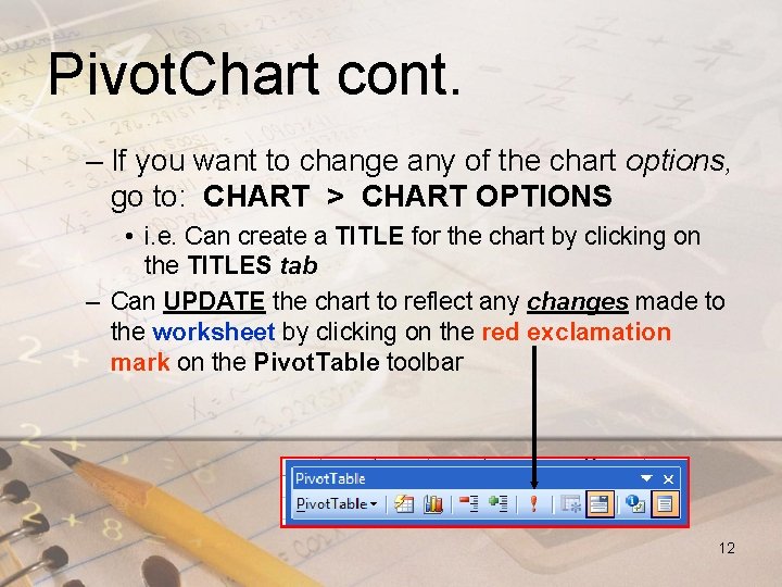
Pivot. Chart cont. – If you want to change any of the chart options, go to: CHART > CHART OPTIONS • i. e. Can create a TITLE for the chart by clicking on the TITLES tab – Can UPDATE the chart to reflect any changes made to the worksheet by clicking on the red exclamation mark on the Pivot. Table toolbar 12