Examples of analyzing MPGD data with emphasis on

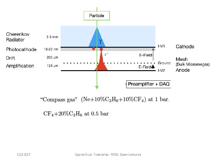
Examples of analyzing MPGD data with emphasis on precise timing 12/13/17 Spyros Eust. Tzamarias - RD 51 Open Lectures

PART I • Prelude • Introduction • Evaluate the number of pes per muon 12/13/17 Spyros Eust. Tzamarias - RD 51 Open Lectures

Prelude 12/13/17 Spyros Eust. Tzamarias - RD 51 Open Lectures

Paradigm: The historian of science Thomas Kuhn gave it its contemporary meaning when he adopted the word to refer to the set of concepts and practices that define a scientific discipline at any particular period of time. In his book The Structure of Scientific Revolutions (first published in 1962), Kuhn defines a scientific paradigm as: "universally recognized scientific achievements that, for a time, provide model problems and solutions for a community of practitioners, i. e. , • what is to be observed and scrutinized • the kind of questions that are supposed to be asked and probed for answers in relation to this subject • how these questions are to be structured • what predictions made by the primary theory within the discipline • how the results of scientific investigations should be interpreted • how an experiment is to be conducted, and what equipment is available to conduct the experiment. Paradigm comes from Greek παράδειγμα (paradeigma), "pattern, example, sample” from the verb παραδείκνυμι (paradeiknumi), "exhibit, represent, expose" and that from παρά (para), "beside, beyond" and δείκνυμι (deiknumi), "to show, to point out" Examples of analyzing MPGD data with emphasis on precise timing 12/13/17 Spyros Eust. Tzamarias - RD 51 Open Lectures

Introduction 12/13/17 Spyros Eust. Tzamarias - RD 51 Open Lectures

12/13/17 Spyros Eust. Tzamarias - RD 51 Open Lectures

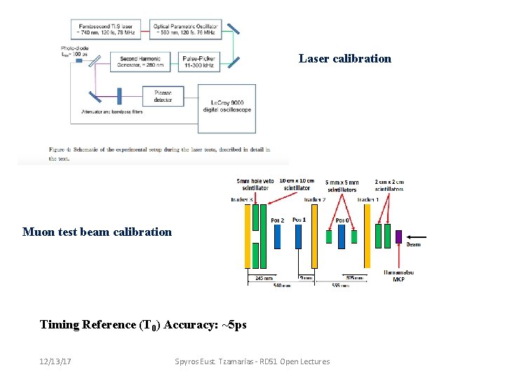
Laser calibration Muon test beam calibration Timing Reference (T 0) Accuracy: ~5 ps 12/13/17 Spyros Eust. Tzamarias - RD 51 Open Lectures

12/13/17 Spyros Eust. Tzamarias - RD 51 Open Lectures

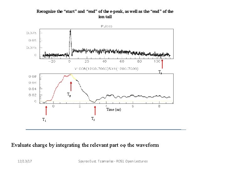
Recognize the “start” and “end” of the e-peak, as well as the “end” of the ion tail T 3 Tp Time (ns) T 1 T 2 Evaluate charge by integrating the relevant part oφ the waveform 12/13/17 Spyros Eust. Tzamarias - RD 51 Open Lectures

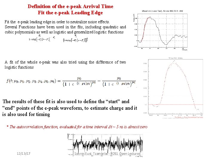
Definition of the e-peak Arrival Time Fit the e-peak Leading Edge Fit the e-peak leading edge in order to neutralize noise effects. Several Functions have been used in the fits, including quadratic and cubic polynomials as well as logistic and generalized logistic functions A fit of the whole e-peak was also tried using the difference of two logistic functions (it is used by K. Paraschou to describe the signal in the simulation of the PICOSEC-MICROMEGAS response) The results of these fit is also used to define the “start” and ”end” points of the e-peak waveform, to estimate charge and it is also used for timing * The autocorrelation function, evaluated for a time interval Δt ~ 5 ns is almost zero 12/13/17 Spyros Eust. Tzamarias - RD 51 Open Lectures

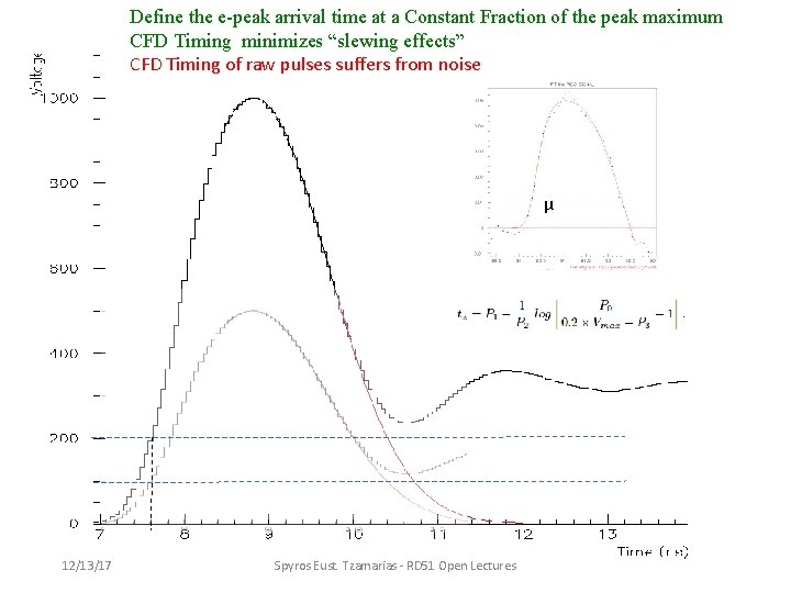
Define the e-peak arrival time at a Constant Fraction of the peak maximum CFD Timing minimizes “slewing effects” CFD Timing of raw pulses suffers from noise μ 12/13/17 Spyros Eust. Tzamarias - RD 51 Open Lectures

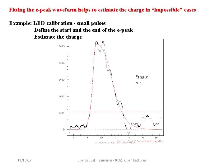
Fitting the e-peak waveform helps to estimate the charge in “impossible” cases Example: LED calibration – small pulses Define the start and the end of the e-peak Estimate the charge Single p. e. 12/13/17 Spyros Eust. Tzamarias - RD 51 Open Lectures

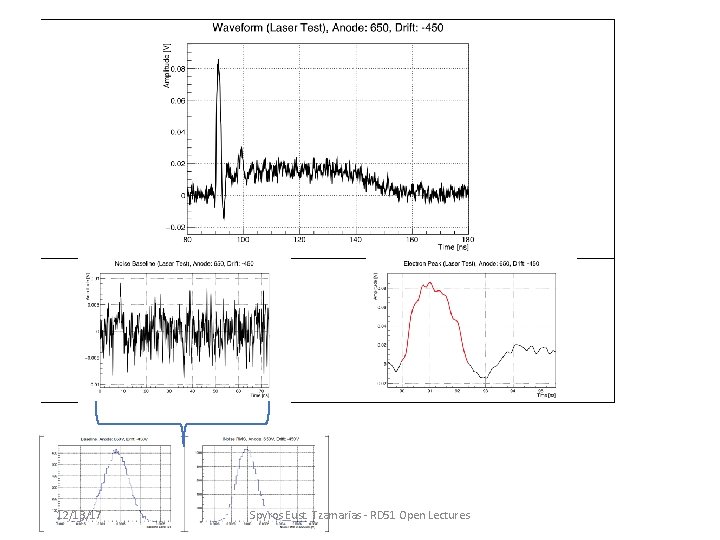
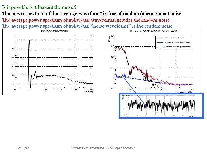
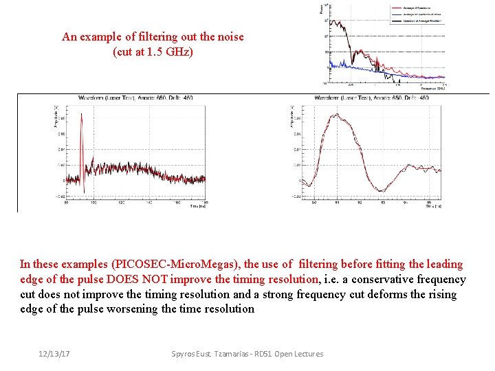
Is it possible to filter-out the noise ? The power spectrum of the “average waveform” is free of random (uncorrelated) noise The average power spectrum of individual waveforms includes the random noise The average power spectrum of individual “noise waveforms” is the random noise 12/13/17 Spyros Eust. Tzamarias - RD 51 Open Lectures

An example of filtering out the noise (cut at 1. 5 GHz) In these examples (PICOSEC-Micro. Megas), the use of filtering before fitting the leading edge of the pulse DOES NOT improve the timing resolution, i. e. a conservative frequency cut does not improve the timing resolution and a strong frequency cut deforms the rising edge of the pulse worsening the time resolution 12/13/17 Spyros Eust. Tzamarias - RD 51 Open Lectures

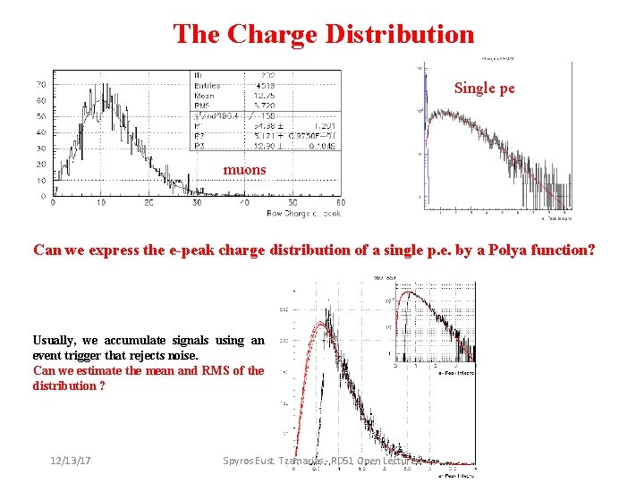
The Charge Distribution Single pe muons Can we express the e-peak charge distribution of a single p. e. by a Polya function? Usually, we accumulate signals using an event trigger that rejects noise. Can we estimate the mean and RMS of the distribution ? 12/13/17 Spyros Eust. Tzamarias - RD 51 Open Lectures

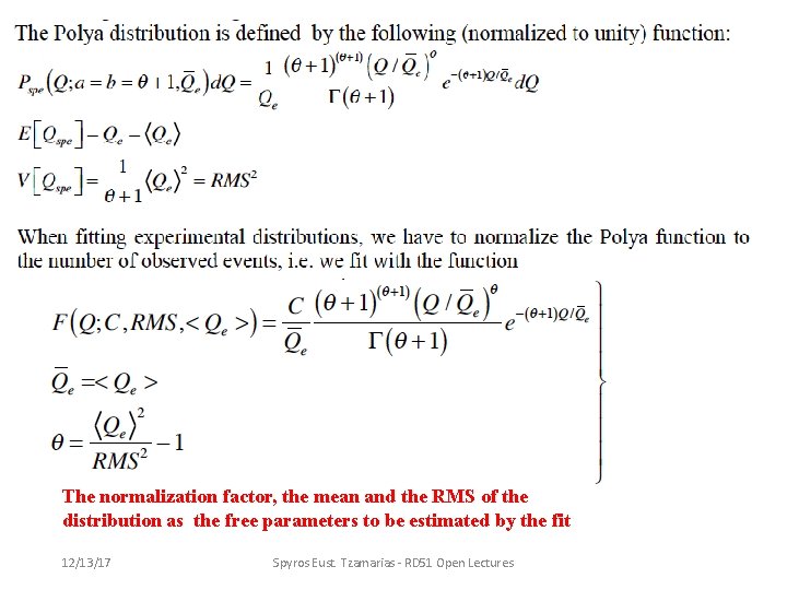
The normalization factor, the mean and the RMS of the distribution as the free parameters to be estimated by the fit 12/13/17 Spyros Eust. Tzamarias - RD 51 Open Lectures

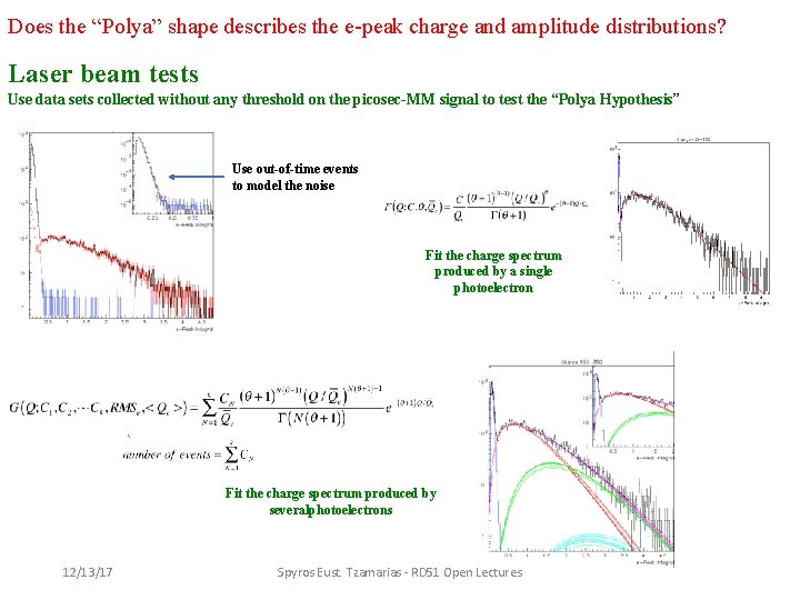
Does the “Polya” shape describes the e-peak charge and amplitude distributions? Laser beam tests Use data sets collected without any threshold on the picosec-MM signal to test the “Polya Hypothesis” Use out-of-time events to model the noise Fit the charge spectrum produced by a single photoelectron Fit the charge spectrum produced by severalphotoelectrons 12/13/17 Spyros Eust. Tzamarias - RD 51 Open Lectures

Evaluate the mean number of pes per muon The last Christmas ghost 12/13/17 Spyros Eust. Tzamarias - RD 51 Open Lectures

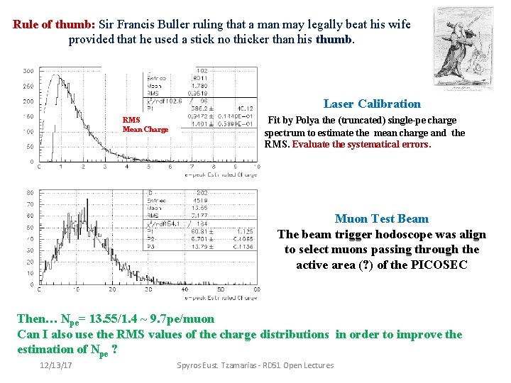
Rule of thumb: Sir Francis Buller ruling that a man may legally beat his wife provided that he used a stick no thicker than his thumb. Laser Calibration RMS Mean Charge Fit by Polya the (truncated) single-pe charge spectrum to estimate the mean charge and the RMS. Evaluate the systematical errors. Muon Test Beam The beam trigger hodoscope was align to select muons passing through the active area (? ) of the PICOSEC Then… Npe= 13. 55/1. 4 ~ 9. 7 pe/muon Can I also use the RMS values of the charge distributions in order to improve the estimation of Npe ? 12/13/17 Spyros Eust. Tzamarias - RD 51 Open Lectures

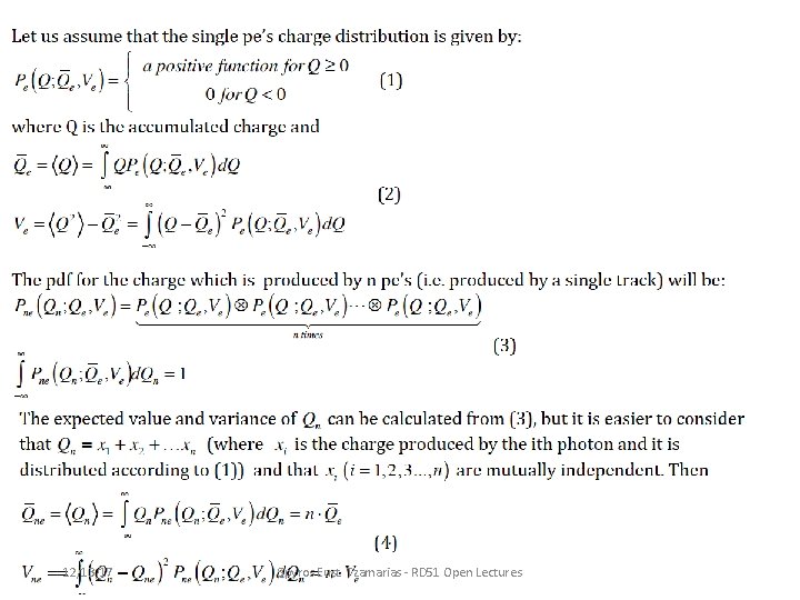
12/13/17 Spyros Eust. Tzamarias - RD 51 Open Lectures

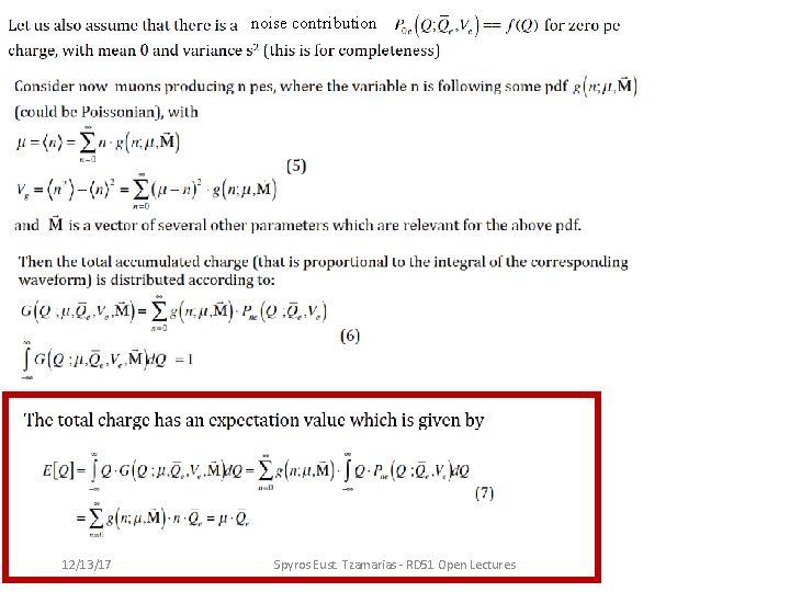
noise contribution 12/13/17 Spyros Eust. Tzamarias - RD 51 Open Lectures

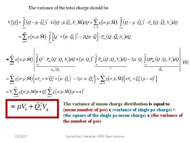
The variance of muon charge distribution is equal to (mean number of pes) x (variance of single pe charge) + (the square of the single pe mean charge) x (the variance of the number of pes) 12/13/17 Spyros Eust. Tzamarias - RD 51 Open Lectures

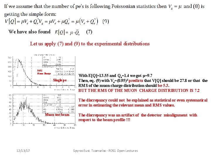
We have also found (7) Let us apply (7) and (9) to the experimental distributions RMS Mean Charge Single pe With E[Q]=13. 55 and Qe=1. 4 we gοt μ=9. 7 Then, eq. (9) with Ve=(0. 95)2 predicts that V[Q] should be 27. 8 or that the RMS of the muon charge distribution should be 5. 3. BUT THE RMS OF THE MUON CHARGE DISTRIBUTION IS 7. 2 The discrepancy could not be explained as statistical or even systematical error in estimating the relevant mean and RMS values. Muon test beam 12/13/17 The discrepancy was an artifact of the detector misalignment with respect to the beam profile !!! Spyros Eust. Tzamarias - RD 51 Open Lectures

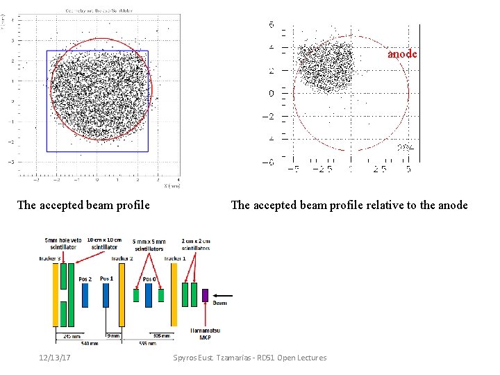
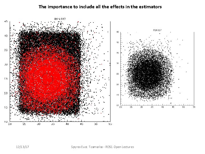
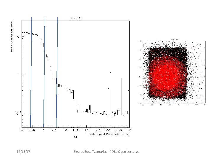
anode The accepted beam profile 12/13/17 The accepted beam profile relative to the anode Spyros Eust. Tzamarias - RD 51 Open Lectures

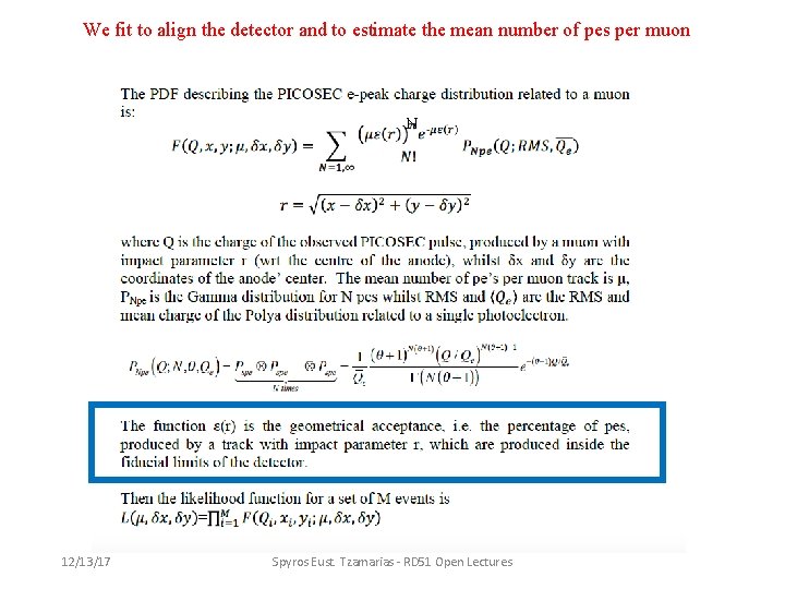
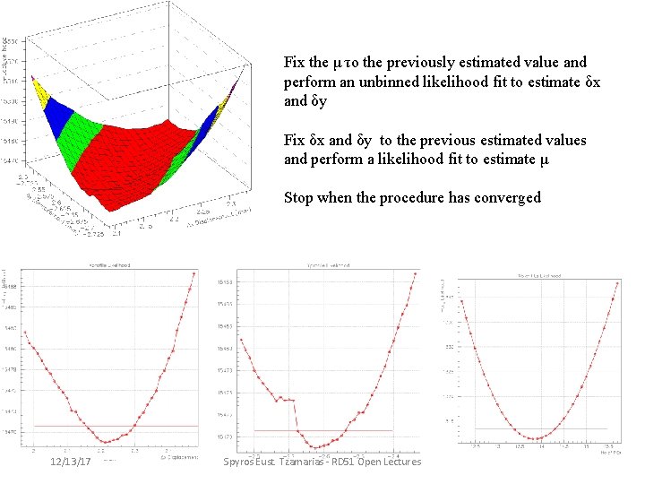
We fit to align the detector and to estimate the mean number of pes per muon N 12/13/17 Spyros Eust. Tzamarias - RD 51 Open Lectures

Fix the μ το the previously estimated value and perform an unbinned likelihood fit to estimate δx and δy Fix δx and δy to the previous estimated values and perform a likelihood fit to estimate μ Stop when the procedure has converged 12/13/17 Spyros Eust. Tzamarias - RD 51 Open Lectures

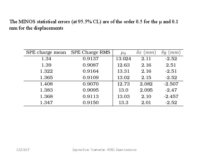
The MINOS statistical errors (at 95. 5% CL) are of the order 0. 5 for the μ and 0. 1 mm for the displacements 12/13/17 Spyros Eust. Tzamarias - RD 51 Open Lectures

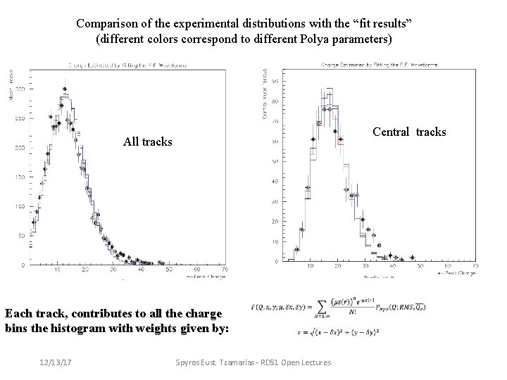
Comparison of the experimental distributions with the “fit results” (different colors correspond to different Polya parameters) Central tracks All tracks Each track, contributes to all the charge bins the histogram with weights given by: 12/13/17 Spyros Eust. Tzamarias - RD 51 Open Lectures

The importance to include all the effects in the estimators 12/13/17 Spyros Eust. Tzamarias - RD 51 Open Lectures

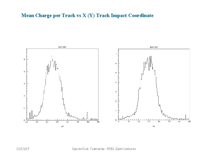
Mean Charge per Track vs X (Y) Track Impact Coordinate 12/13/17 Spyros Eust. Tzamarias - RD 51 Open Lectures

12/13/17 Spyros Eust. Tzamarias - RD 51 Open Lectures

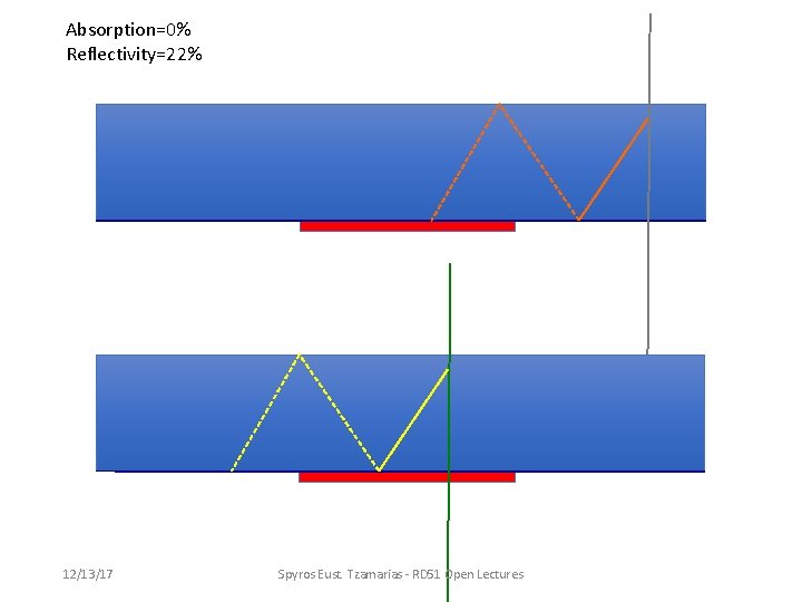
Absorption=0% Reflectivity=22% 12/13/17 Spyros Eust. Tzamarias - RD 51 Open Lectures

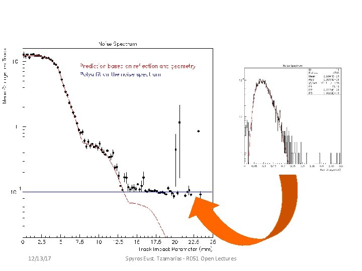
12/13/17 Spyros Eust. Tzamarias - RD 51 Open Lectures