Examples and applications of discrete dynamical systems in

Examples and applications of discrete dynamical systems in economic, social and ecological systems Fabio Tramontana

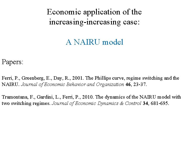
Economic application of the increasing-increasing case: A NAIRU model Papers: Ferri, P. , Greenberg, E. , Day, R. , 2001. The Phillips curve, regime switching and the NAIRU. Journal of Economic Behavior and Organization 46, 23 -37. Tramontana, F. , Gardini, L. , Ferri, P. , 2010. The dynamics of the NAIRU model with two switching regimes. Journal of Economic Dynamics & Control 34, 681 -695.

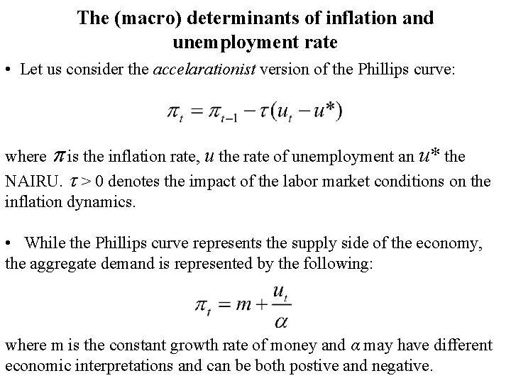
The (macro) determinants of inflation and unemployment rate • Let us consider the accelarationist version of the Phillips curve: where is the inflation rate, u the rate of unemployment an u* the NAIRU. > 0 denotes the impact of the labor market conditions on the inflation dynamics. • While the Phillips curve represents the supply side of the economy, the aggregate demand is represented by the following: where m is the constant growth rate of money and α may have different economic interpretations and can be both postive and negative.

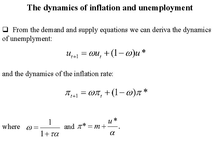
The dynamics of inflation and unemployment q From the demand supply equations we can deriva the dynamics of unemplyment: and the dynamics of the inflation rate: where and

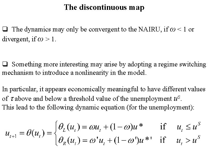
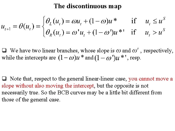
The discontinuous map q The dynamics may only be convergent to the NAIRU, if ω < 1 or divergent, if ω > 1. q Something more interesting may arise by adopting a regime switching mechanism to introduce a nonlinearity in the model. In particular, it appears economically meaningful to have different values of above and below a threshold value of the unemployment u. S. This lead to the following dynamic equation (for the unemployment):

The discontinuous map q We have two linear branches, whose slope is ω and ω′ , respectively, while the intercepts are and , resp. q Note that, respect to the general linear-linear case, you cannot move a slope without also moving the intercept, but the opposite is not necessarily true. So the BCB curves may be a little bit different from those of the general case.

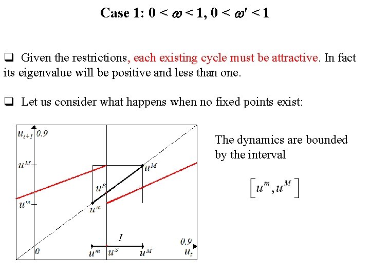
Case 1: 0 < < 1, 0 < ′ < 1 q Given the restrictions, each existing cycle must be attractive. In fact its eigenvalue will be positive and less than one. q Let us consider what happens when no fixed points exist: The dynamics are bounded by the interval

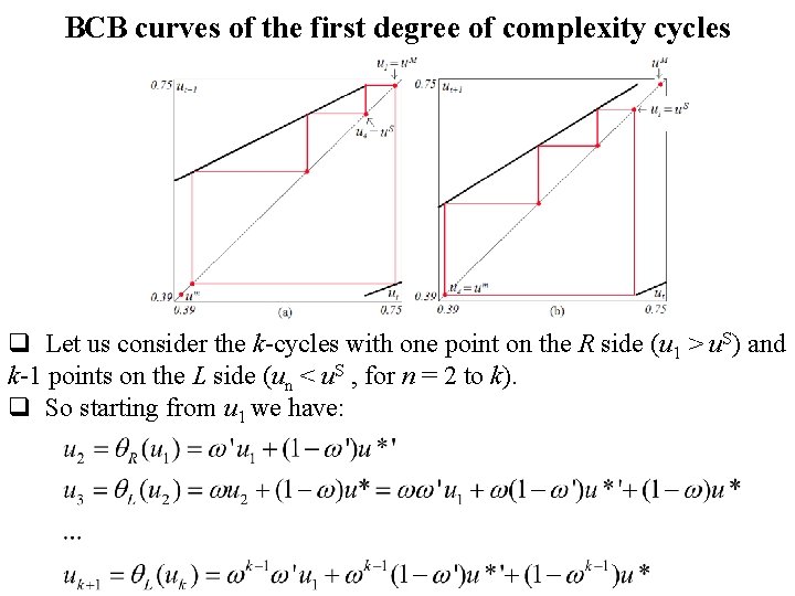
BCB curves of the first degree of complexity cycles q Let us consider the k-cycles with one point on the R side (u 1 > u. S) and k-1 points on the L side (un < u. S , for n = 2 to k). q So starting from u 1 we have:

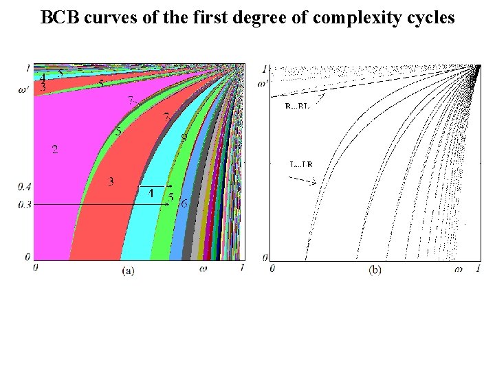
BCB curves of the first degree of complexity cycles q We have a k-cycle belonging to the first complexity level family whenever uk+1 = u 1, that is: and by iterating u 1, we also obtain: q The BCB are obtained by using the conditions u 1 = us and uk = us :

BCB curves of the first degree of complexity cycles

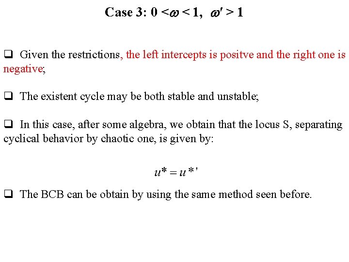
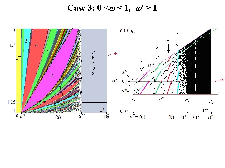
Case 3: 0 < < 1, ′ > 1 q Given the restrictions, the left intercepts is positve and the right one is negative; q The existent cycle may be both stable and unstable; q In this case, after some algebra, we obtain that the locus S, separating cyclical behavior by chaotic one, is given by: q The BCB can be obtain by using the same method seen before.

Case 3: 0 < < 1, ′ > 1

A three-dimensional Lotka-Volterra model Paper: Bischi, G. I. , Tramontana, 2010. Three-dimensional discrete-time Lotka-Volterra models with an application to industrial clusters. Communications in Nonlinear Science and Numerical Simulation 15, 3000 -3014.

Lotka-Volterra models • Among the most famous biologic applications of dynamical systems, there are the Lotka-Volterra equations; • Starting from the orginal application of Volterra to populations of fishes in the Adriatic see, these models have been applied to several other fields: ü Chemistry (Lotka) ü Economics (Goodwin) ü Social interactions ü Physics

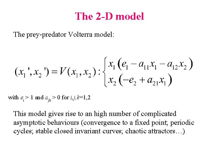
The 2 -D model The prey-predator Volterra model: with ei > 1 and ajk > 0 for i, j, k=1, 2 This model gives rise to an high number of complicated asymptotic behaviours (convergence to a fixed point; periodic cycles; stable closed invariant curves; chaotic attractors…)

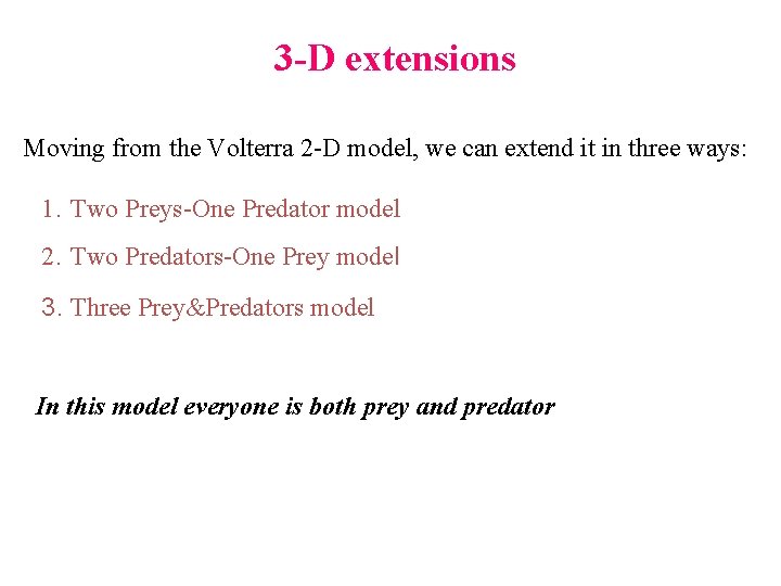
3 -D extensions Moving from the Volterra 2 -D model, we can extend it in three ways: 1. Two Preys-One Predator model 2. Two Predators-One Prey model 3. Three Prey&Predators model In this model everyone is both prey and predator

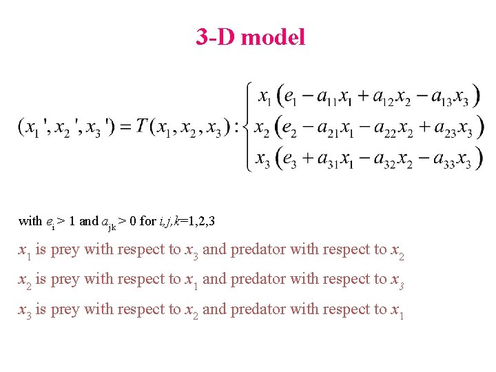
3 -D model with ei > 1 and ajk > 0 for i, j, k=1, 2, 3 x 1 is prey with respect to x 3 and predator with respect to x 2 is prey with respect to x 1 and predator with respect to x 3 is prey with respect to x 2 and predator with respect to x 1

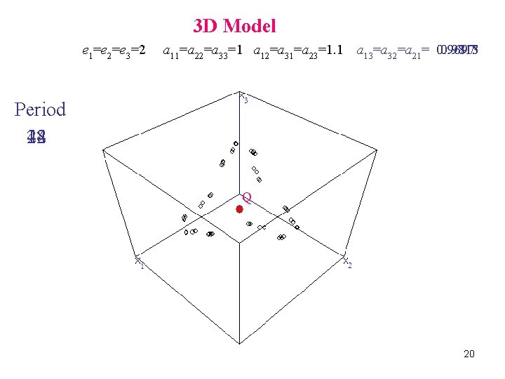
Fixed points The model has got eight fixed points: O(0, 0, 0) extinction of all groups (never stable) Ei for i = 1, 2, 3 only one group survives Eij for i=2, 3 j=1, 2 and i > j Q two groups survive three-groups equilibrium

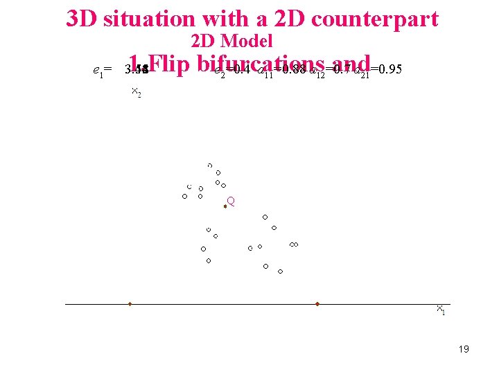
3 D situation with a 2 D counterpart 2 D Model 1. Flip bifurcations and e =0. 4 a =0. 88 a =0. 7 a =0. 95 e 1= 3. 54 3. 52 3. 5 3. 48 3. 55 2 11 12 21 Periodic cycles Q 19

3 D Model e 1=e 2=e 3=2 a 11=a 22=a 33=1 a 12=a 31=a 23=1. 1 a 13=a 32=a 21= 0. 9697 0. 98 0. 9713 0. 9715 Period 12 48 24 Q 20

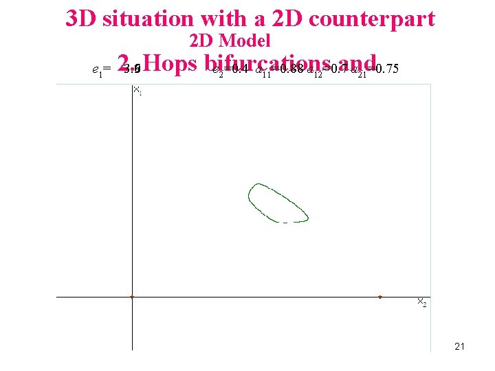
3 D situation with a 2 D counterpart 2 D Model 2. Hops bifurcations and e =0. 4 a =0. 88 a =0. 75 e 1= 3. 9 3. 6 2 11 12 21 Invariant closed curves 21

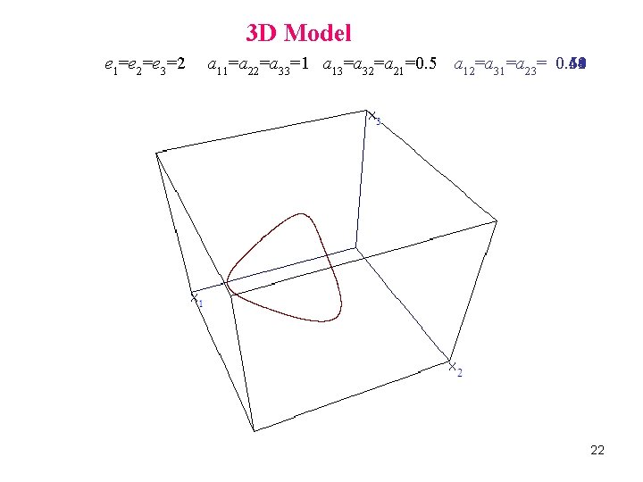
3 D Model e 1=e 2=e 3=2 a 11=a 22=a 33=1 a 13=a 32=a 21=0. 5 a 12=a 31=a 23= 0. 58 0. 44 0. 61 0. 59 Q 22

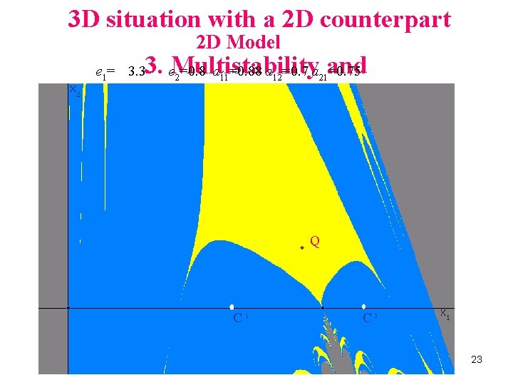
3 D situation with a 2 D counterpart 2 D Model 3. e. Multistability =0. 8 a =0. 88 a =0. 7 a and =0. 75 e 1= 3. 3 2 11 12 21 Path Dependence Q C 1 C 2 23

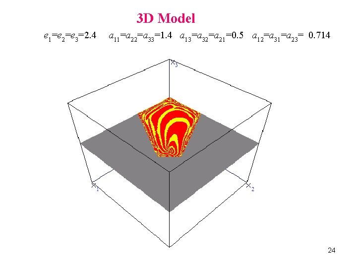
3 D Model e 1=e 2=e 3=2. 4 a 11=a 22=a 33=1. 4 a 13=a 32=a 21=0. 5 a 12=a 31=a 23= 0. 714 24

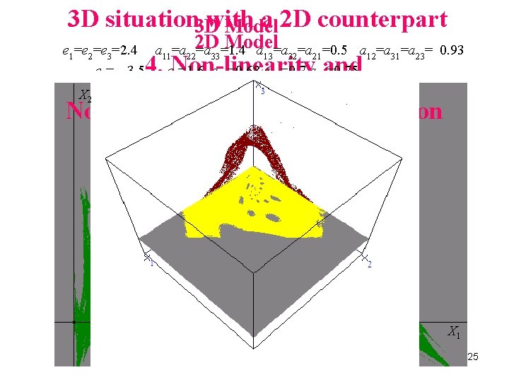
3 D situation 3 D with a 2 D counterpart Model e 1=e 2=e 3=2. 4 a 11=a 222 D =a 33=1. 4 a 13=a 32=a 21=0. 5 a 12=a 31=a 23= 0. 93 e 1= 3. 5 e 2=1. 6 a 11=0. 68 a 12=0. 7 a 21=0. 75 4. Non-linearity and X 2 Non-connected basins of attraction X 1 25

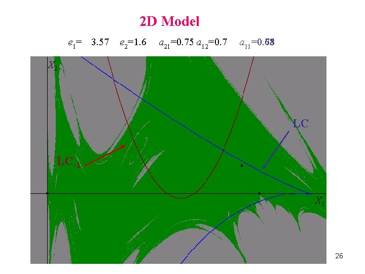
2 D Model e 1= 3. 57 e 2=1. 6 a 21=0. 75 a 12=0. 7 a 11=0. 68 =0. 75 =0. 73 =0. 7 X 2 LC LC-1 X 1 26

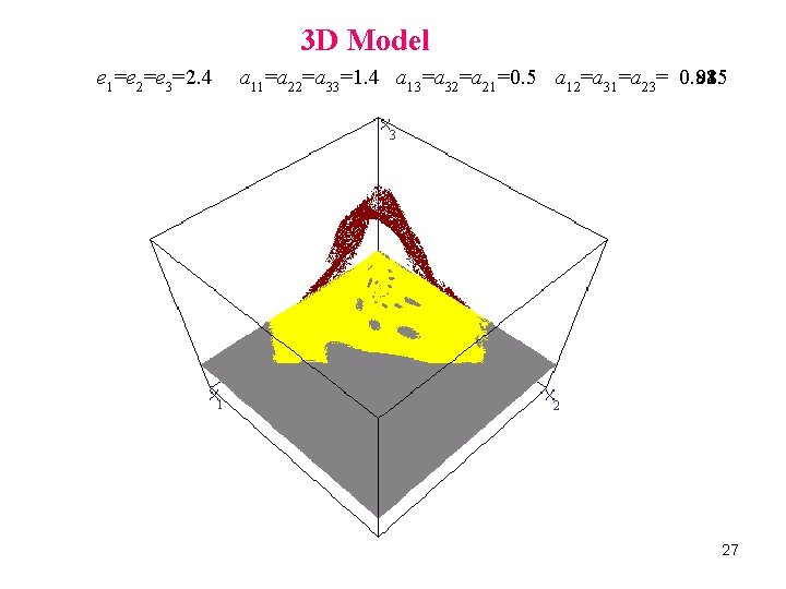
3 D Model e 1=e 2=e 3=2. 4 a 11=a 22=a 33=1. 4 a 13=a 32=a 21=0. 5 a 12=a 31=a 23= 0. 885 0. 93 0. 92 0. 91 3 1 2 27

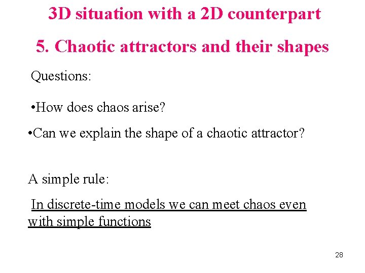
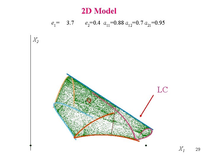
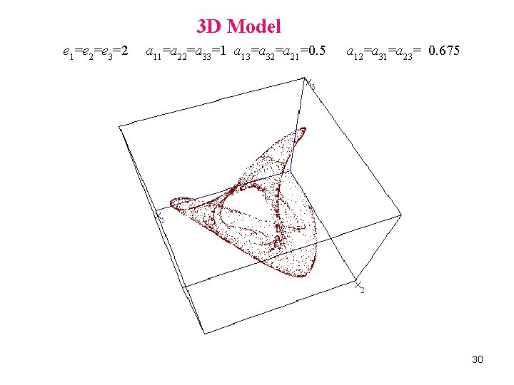
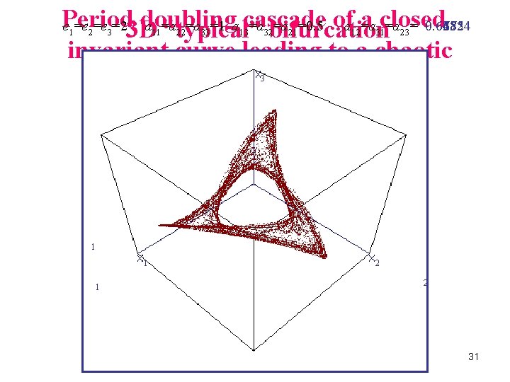
3 D situation with a 2 D counterpart 5. Chaotic attractors and their shapes Questions: • How does chaos arise? • Can we explain the shape of a chaotic attractor? A simple rule: In discrete-time models we can meet chaos even with simple functions 28

2 D Model e 1 = 3. 7 e 2=0. 4 a 11=0. 88 a 12=0. 7 a 21=0. 95 X 2 LC-1 LC Q Q X 1 29

3 D Model e 1=e 2=e 3=2 a 11=a 22=a 33=1 a 13=a 32=a 21=0. 5 a 12=a 31=a 23= 0. 675 30

Period doubling cascade of a closed a =a 0. 675 0. 67 0. 66824 0. 665 0. 66 0. 658 0. 6575 0. 64 0. 63 e =e =e =23 D a =a =a =1 a =a =a =0. 5 “typical” bifurcation=a = 0. 62 invariant curve leading to a chaotic attractor 1 2 3 11 22 33 13 32 21 12 31 23 3 1 1 1 2 2 31

An application of discrete dynamical systems in Game Theory: The Cournot duopoly model with isoelastic demand constant unit costs Papers: Puu, T. , 1991. Chaos in duopoly pricing. Chaos, Solitons & Fractals 1, 573 -581. Bischi, G. I. , Mammana, C. , Gardini, L. , 2000. Multistability and cyclic attractors in duopoly games. Chaos, Solitons & Fractals 11, 543 -564. Tramontana, F. , Gardini, L. , Puu, T. , 2010. New properties of the Cournot duopoly with isoelastic demand constant unit costs. Submitted.

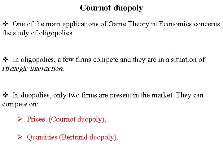
Cournot duopoly v One of the main applications of Game Theory in Economics concerns the study of oligopolies. v In oligopolies, a few firms compete and they are in a situation of strategic interaction. v In duopolies, only two firms are present in the market. They can compete on: Ø Prices (Cournot duopoly); Ø Quantities (Bertrand duopoly).

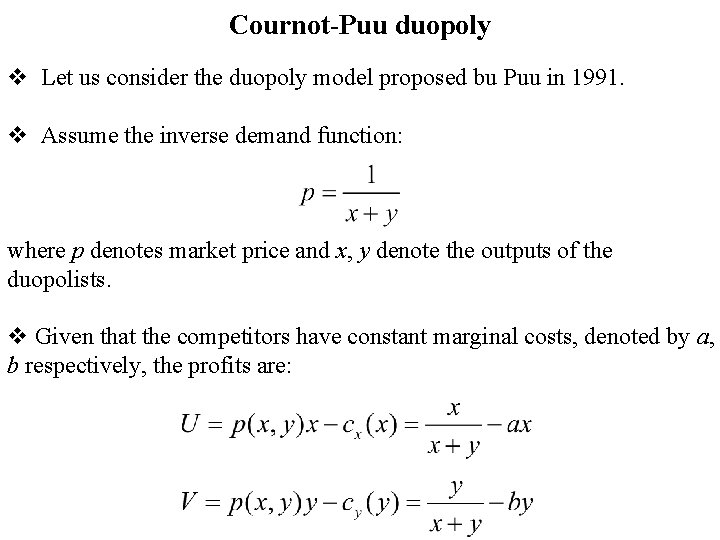
Cournot-Puu duopoly v Let us consider the duopoly model proposed bu Puu in 1991. v Assume the inverse demand function: where p denotes market price and x, y denote the outputs of the duopolists. v Given that the competitors have constant marginal costs, denoted by a, b respectively, the profits are:

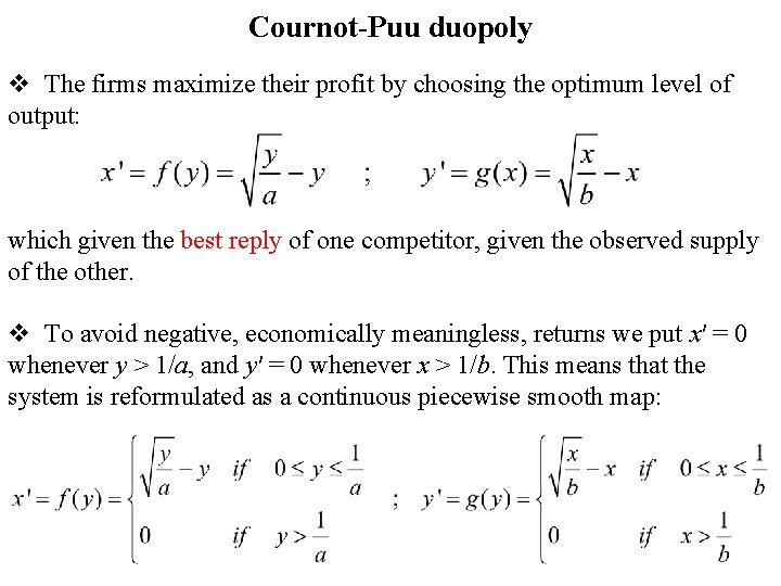
Cournot-Puu duopoly v The firms maximize their profit by choosing the optimum level of output: which given the best reply of one competitor, given the observed supply of the other. v To avoid negative, economically meaningless, returns we put x′ = 0 whenever y > 1/a, and y′ = 0 whenever x > 1/b. This means that the system is reformulated as a continuous piecewise smooth map:

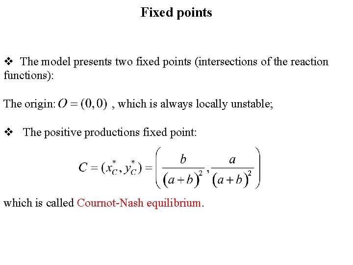
Fixed points v The model presents two fixed points (intersections of the reaction functions): The origin: , which is always locally unstable; v The positive productions fixed point: which is called Cournot-Nash equilibrium.

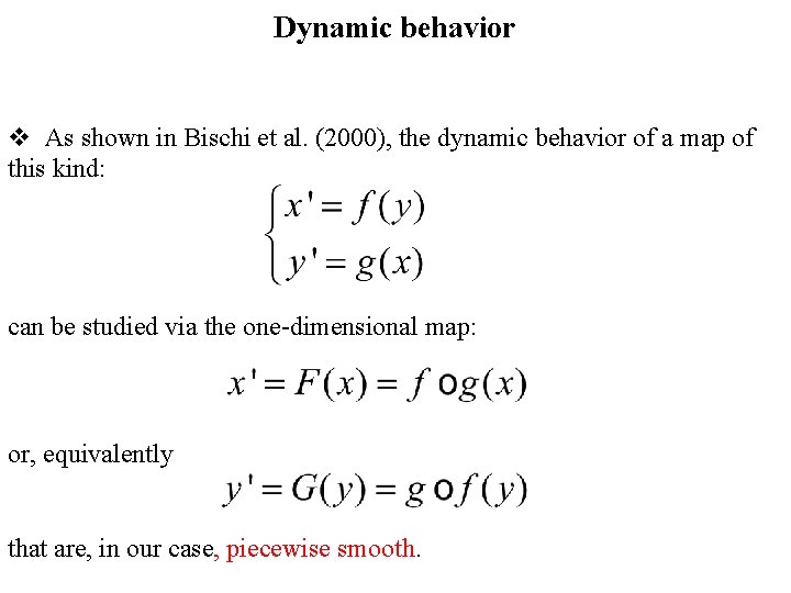
Dynamic behavior v As shown in Bischi et al. (2000), the dynamic behavior of a map of this kind: can be studied via the one-dimensional map: or, equivalently that are, in our case, piecewise smooth.

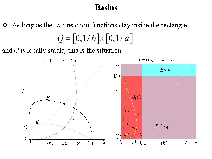
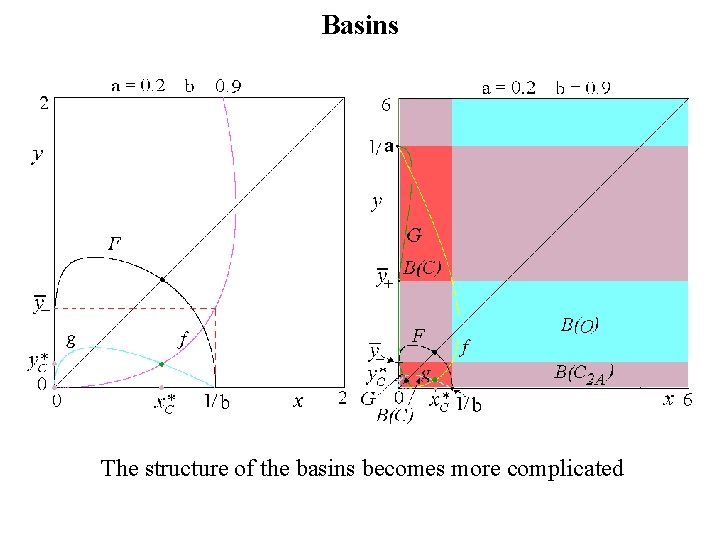
Basins v As long as the two reaction functions stay inside the rectangle: and C is locally stable, this is the situation:

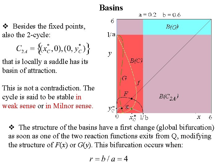
Basins v Besides the fixed points, also the 2 -cycle: that is locally a saddle has its basin of attraction. This is not a contradiction. The cycle is said to be stable in weak sense or in Milnor sense. v The structure of the basins have a first change (global bifurcation) as soon as one of the two reaction functions exits from Q, modifying the structure of F(x) or G(y). This bifurcation occurs when:

Basins The structure of the basins becomes more complicated

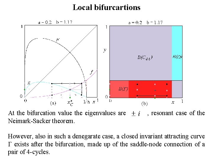
Local bifurcartions A flip-bifurcation of the map F(x) corresponds to a degenerate Neimark. Sacher bifurcation for T. The Jacobian matrix of our map T in the smooth branches, evaluated in the Cournot-Nash fixed point is given by: and its characteristic polynomial is given by: Thus the eigenvalues are pure imaginary and the equilibrium is stable as long as , which occurs as long as:

Local bifurcartions At the bifurcation value the eigenvalues are Neimark-Sacker theorem. , resonant case of the However, also in such a denegarate case, a closed invariant attracting curve exists after the bifurcation, made up of the saddle-node connection of a pair of 4 -cycles.

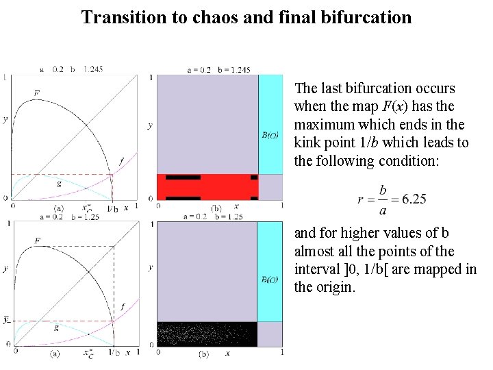
Transition to chaos and final bifurcation The last bifurcation occurs when the map F(x) has the maximum which ends in the kink point 1/b which leads to the following condition: and for higher values of b almost all the points of the interval ]0, 1/b[ are mapped in the origin.

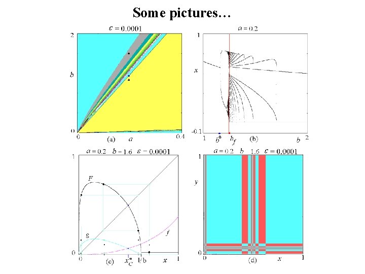
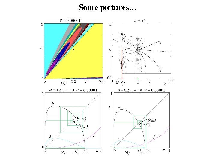
A remedy to undesired festures o The fact that once the zero value is get, the iterated states in the duopoly can no longer abandon the coordinate axes, even if the cycles on the axes are locally unstable; o Thus, a more interesting model, satisfying the intuitive economic behavior, is that a state variable x or y can become very low, assuming a fixed low value, say , after which they can increase again. For sake of simplicity let us take the same constant low value for both the competitors. o We obtain the following piecewise smooth, but now discontinuous map:

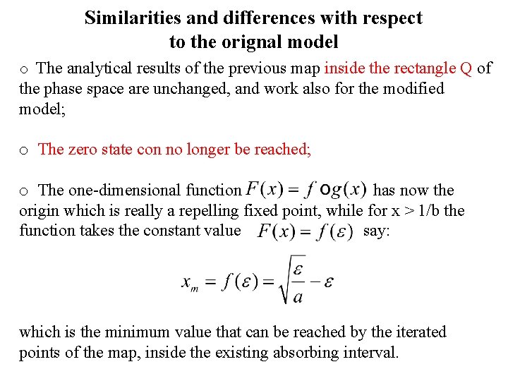
Similarities and differences with respect to the orignal model o The analytical results of the previous map inside the rectangle Q of the phase space are unchanged, and work also for the modified model; o The zero state con no longer be reached; o The one-dimensional function has now the origin which is really a repelling fixed point, while for x > 1/b the function takes the constant value say: which is the minimum value that can be reached by the iterated points of the map, inside the existing absorbing interval.

Some pictures…

Some pictures…

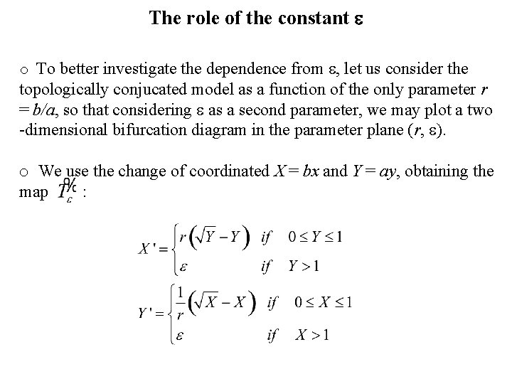
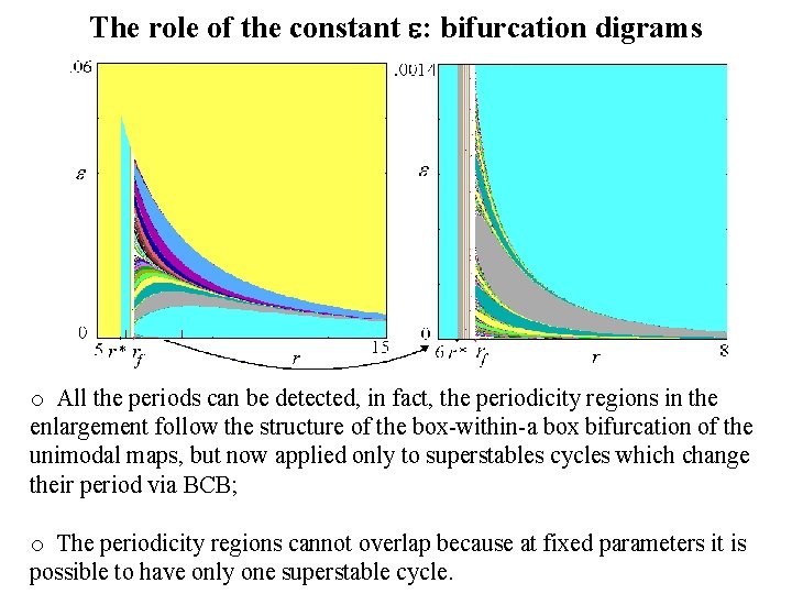
The role of the constant o To better investigate the dependence from , let us consider the topologically conjucated model as a function of the only parameter r = b/a, so that considering as a second parameter, we may plot a two -dimensional bifurcation diagram in the parameter plane (r, ). o We use the change of coordinated X = bx and Y = ay, obtaining the map :

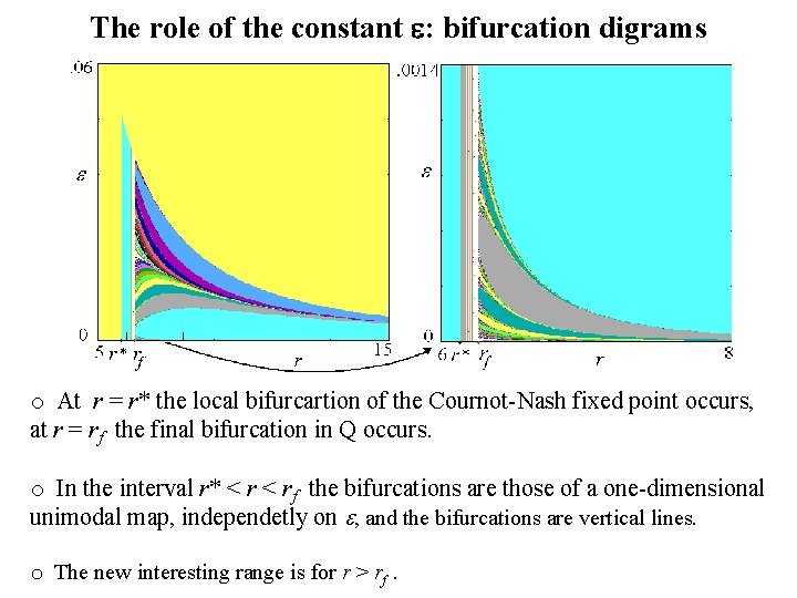
The role of the constant : bifurcation digrams o At r = r* the local bifurcartion of the Cournot-Nash fixed point occurs, at r = rf the final bifurcation in Q occurs. o In the interval r* < rf the bifurcations are those of a one-dimensional unimodal map, independetly on , and the bifurcations are vertical lines. o The new interesting range is for r > rf.

The role of the constant : bifurcation digrams o All the periods can be detected, in fact, the periodicity regions in the enlargement follow the structure of the box-within-a box bifurcation of the unimodal maps, but now applied only to superstables cycles which change their period via BCB; o The periodicity regions cannot overlap because at fixed parameters it is possible to have only one superstable cycle.