Example In a recent poll 70 of 1501

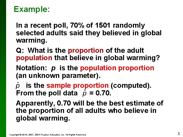
Example: In a recent poll, 70% of 1501 randomly selected adults said they believed in global warming. Q: What is the proportion of the adult population that believe in global warming? Notation: p is the population proportion (an unknown parameter). is the sample proportion (computed). From the poll data = 0. 70. Apparently, 0. 70 will be the best estimate of the proportion of all adults who believe in global warming. Copyright © 2010, 2007, 2004 Pearson Education, Inc. All Rights Reserved. 1

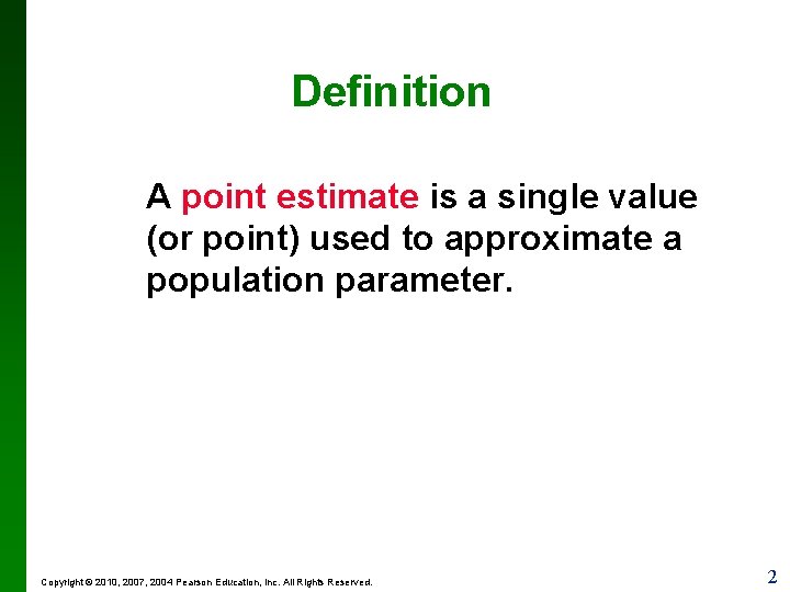
Definition A point estimate is a single value (or point) used to approximate a population parameter. Copyright © 2010, 2007, 2004 Pearson Education, Inc. All Rights Reserved. 2

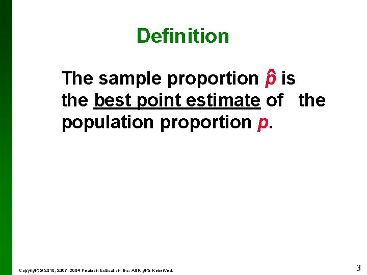
Definition ˆ The sample proportion p is the best point estimate of the population proportion p. Copyright © 2010, 2007, 2004 Pearson Education, Inc. All Rights Reserved. 3

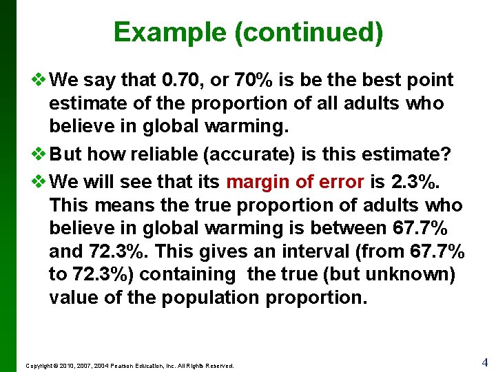
Example (continued) v We say that 0. 70, or 70% is be the best point estimate of the proportion of all adults who believe in global warming. v But how reliable (accurate) is this estimate? v We will see that its margin of error is 2. 3%. This means the true proportion of adults who believe in global warming is between 67. 7% and 72. 3%. This gives an interval (from 67. 7% to 72. 3%) containing the true (but unknown) value of the population proportion. Copyright © 2010, 2007, 2004 Pearson Education, Inc. All Rights Reserved. 4

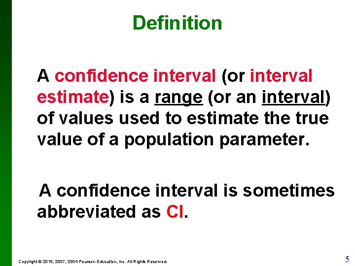
Definition A confidence interval (or interval estimate) is a range (or an interval) of values used to estimate the true value of a population parameter. A confidence interval is sometimes abbreviated as CI. Copyright © 2010, 2007, 2004 Pearson Education, Inc. All Rights Reserved. 5

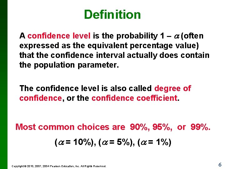
Definition A confidence level is the probability 1 – (often expressed as the equivalent percentage value) that the confidence interval actually does contain the population parameter. The confidence level is also called degree of confidence, or the confidence coefficient. Most common choices are 90%, 95%, or 99%. ( = 10%), ( = 5%), ( = 1%) Copyright © 2010, 2007, 2004 Pearson Education, Inc. All Rights Reserved. 6

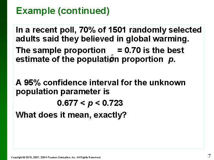
Example (continued) In a recent poll, 70% of 1501 randomly selected adults said they believed in global warming. The sample proportion = 0. 70 is the best estimate of the population proportion p. A 95% confidence interval for the unknown population parameter is 0. 677 < p < 0. 723 What does it mean, exactly? Copyright © 2010, 2007, 2004 Pearson Education, Inc. All Rights Reserved. 7

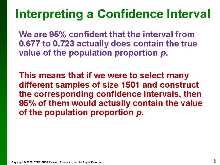
Interpreting a Confidence Interval We are 95% confident that the interval from 0. 677 to 0. 723 actually does contain the true value of the population proportion p. This means that if we were to select many different samples of size 1501 and construct the corresponding confidence intervals, then 95% of them would actually contain the value of the population proportion p. Copyright © 2010, 2007, 2004 Pearson Education, Inc. All Rights Reserved. 8

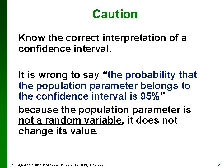
Caution Know the correct interpretation of a confidence interval. It is wrong to say “the probability that the population parameter belongs to the confidence interval is 95%” because the population parameter is not a random variable, it does not change its value. Copyright © 2010, 2007, 2004 Pearson Education, Inc. All Rights Reserved. 9

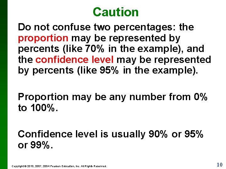
Caution Do not confuse two percentages: the proportion may be represented by percents (like 70% in the example), and the confidence level may be represented by percents (like 95% in the example). Proportion may be any number from 0% to 100%. Confidence level is usually 90% or 95% or 99%. Copyright © 2010, 2007, 2004 Pearson Education, Inc. All Rights Reserved. 10

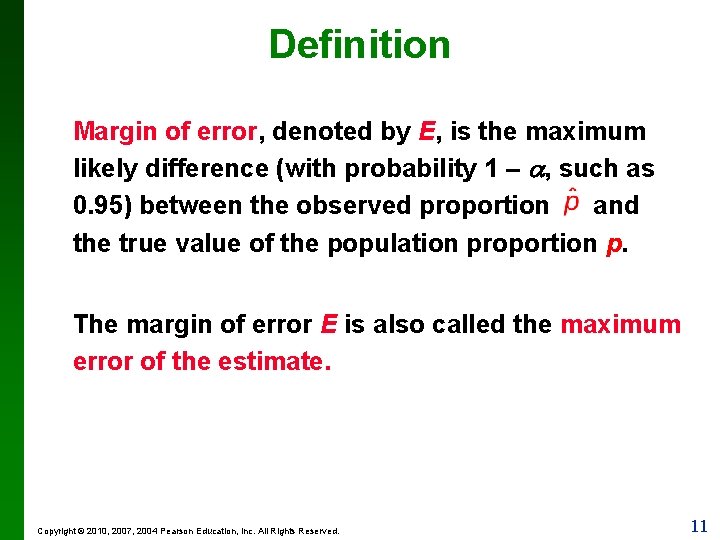
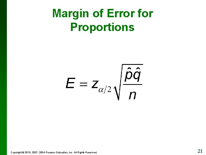
Definition Margin of error, denoted by E, is the maximum likely difference (with probability 1 – , such as 0. 95) between the observed proportion and the true value of the population proportion p. The margin of error E is also called the maximum error of the estimate. Copyright © 2010, 2007, 2004 Pearson Education, Inc. All Rights Reserved. 11

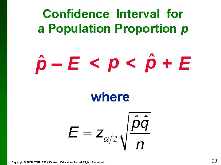
Confidence Interval for a Population Proportion p ˆ – E < pˆ + E p ˆ + E) (pˆ – E, p Copyright © 2010, 2007, 2004 Pearson Education, Inc. All Rights Reserved. 12

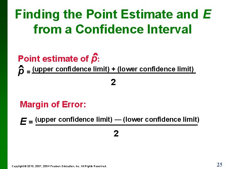
Finding the Point Estimate and E from a Confidence Interval ˆ (upper confidence limit) + (lower confidence limit) Point estimate of p: ˆ p= 2 Margin of Error: E = (upper confidence limit) — (lower confidence limit) 2 Copyright © 2010, 2007, 2004 Pearson Education, Inc. All Rights Reserved. 13

Next we learn how to construct confidence intervals Copyright © 2010, 2007, 2004 Pearson Education, Inc. All Rights Reserved. 14

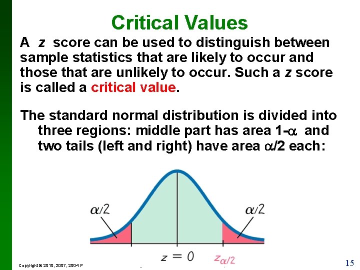
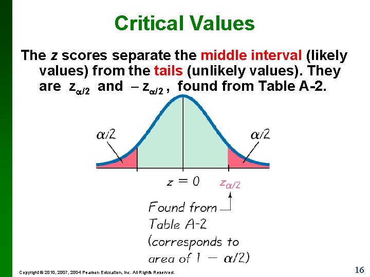
Critical Values A z score can be used to distinguish between sample statistics that are likely to occur and those that are unlikely to occur. Such a z score is called a critical value. The standard normal distribution is divided into three regions: middle part has area 1 -a and two tails (left and right) have area a/2 each: Copyright © 2010, 2007, 2004 Pearson Education, Inc. All Rights Reserved. 15

Critical Values The z scores separate the middle interval (likely values) from the tails (unlikely values). They are za/2 and – za/2 , found from Table A-2. Copyright © 2010, 2007, 2004 Pearson Education, Inc. All Rights Reserved. 16

Definition A critical value is the number on the borderline separating sample statistics that are likely to occur from those that are unlikely to occur. Copyright © 2010, 2007, 2004 Pearson Education, Inc. All Rights Reserved. 17

Notation for Critical Value The critical value z /2 separates an area of /2 in the right tail of the standard normal distribution. The value of –z /2 separates an area of /2 in the left tail. The subscript /2 is simply a reminder that the z score separates an area of /2 in the tail. Copyright © 2010, 2007, 2004 Pearson Education, Inc. All Rights Reserved. 18

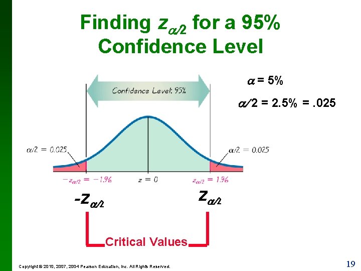
Finding z 2 for a 95% Confidence Level = 5% 2 = 2. 5% =. 025 z 2 -z 2 Critical Values Copyright © 2010, 2007, 2004 Pearson Education, Inc. All Rights Reserved. 19

Definition Margin of error, denoted by E, is the maximum likely difference (with probability 1 – , such as 0. 95) between the observed proportion and the true value of the population proportion p. The margin of error E is also called the maximum error of the estimate. Copyright © 2010, 2007, 2004 Pearson Education, Inc. All Rights Reserved. 20

Margin of Error for Proportions Copyright © 2010, 2007, 2004 Pearson Education, Inc. All Rights Reserved. 21

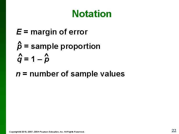
Notation E = margin of error ^ = sample proportion p q^ = 1 – ^ p n = number of sample values Copyright © 2010, 2007, 2004 Pearson Education, Inc. All Rights Reserved. 22

Confidence Interval for a Population Proportion p pˆ – E < pˆ + E where Copyright © 2010, 2007, 2004 Pearson Education, Inc. All Rights Reserved. 23

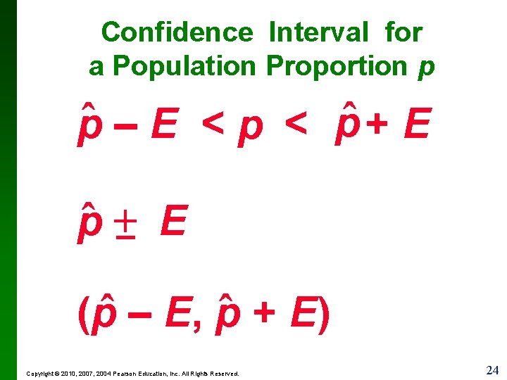
Confidence Interval for a Population Proportion p ˆ – E < pˆ + E p ˆ + E) (pˆ – E, p Copyright © 2010, 2007, 2004 Pearson Education, Inc. All Rights Reserved. 24

Finding the Point Estimate and E from a Confidence Interval ˆ (upper confidence limit) + (lower confidence limit) Point estimate of p: ˆ p= 2 Margin of Error: E = (upper confidence limit) — (lower confidence limit) 2 Copyright © 2010, 2007, 2004 Pearson Education, Inc. All Rights Reserved. 25

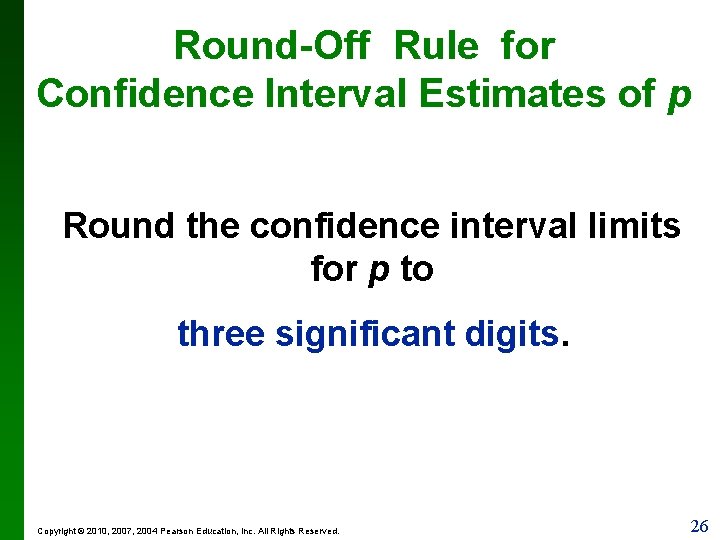
Round-Off Rule for Confidence Interval Estimates of p Round the confidence interval limits for p to three significant digits. Copyright © 2010, 2007, 2004 Pearson Education, Inc. All Rights Reserved. 26

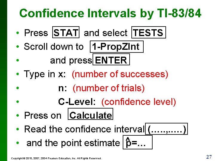
Confidence Intervals by TI-83/84 • • • Press STAT and select TESTS Scroll down to 1 -Prop. ZInt and press ENTER Type in x: (number of successes) n: (number of trials) C-Level: (confidence level) Press on Calculate Read the confidence interval (…. . , . . …) and the point estimate ^ p=… Copyright © 2010, 2007, 2004 Pearson Education, Inc. All Rights Reserved. 27

Sample Size Suppose we want to collect sample data in order to estimate some population proportion. The question is how many sample items must be obtained? Copyright © 2010, 2007, 2004 Pearson Education, Inc. All Rights Reserved. 28

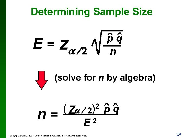
Determining Sample Size z 2 E= p ˆ qˆ n (solve for n by algebra) n= ( Z 2 )2 p ˆ ˆq E 2 Copyright © 2010, 2007, 2004 Pearson Education, Inc. All Rights Reserved. 29

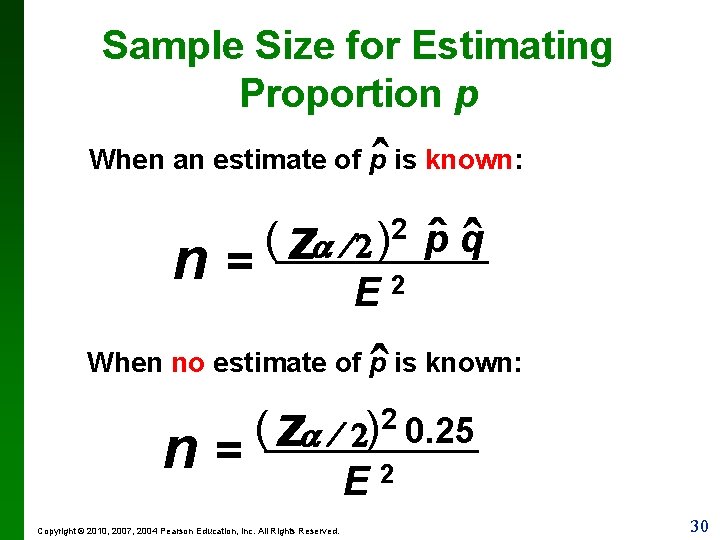
Sample Size for Estimating Proportion p ˆ When an estimate of p is known: n= ( z 2 pˆ qˆ 2 ) E 2 ˆ When no estimate of p is known: n= ( z 2) 2 0. 25 Copyright © 2010, 2007, 2004 Pearson Education, Inc. All Rights Reserved. E 2 30

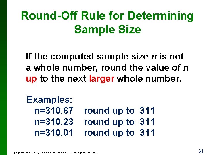
Round-Off Rule for Determining Sample Size If the computed sample size n is not a whole number, round the value of n up to the next larger whole number. Examples: n=310. 67 n=310. 23 n=310. 01 round up to 311 Copyright © 2010, 2007, 2004 Pearson Education, Inc. All Rights Reserved. 31

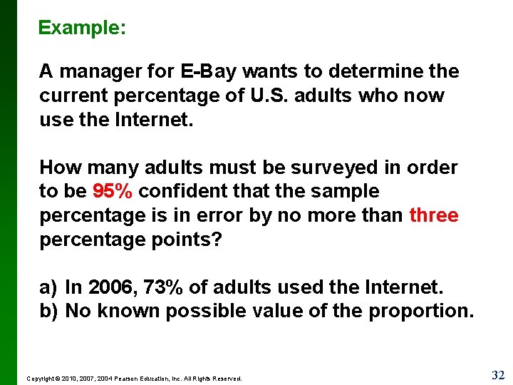
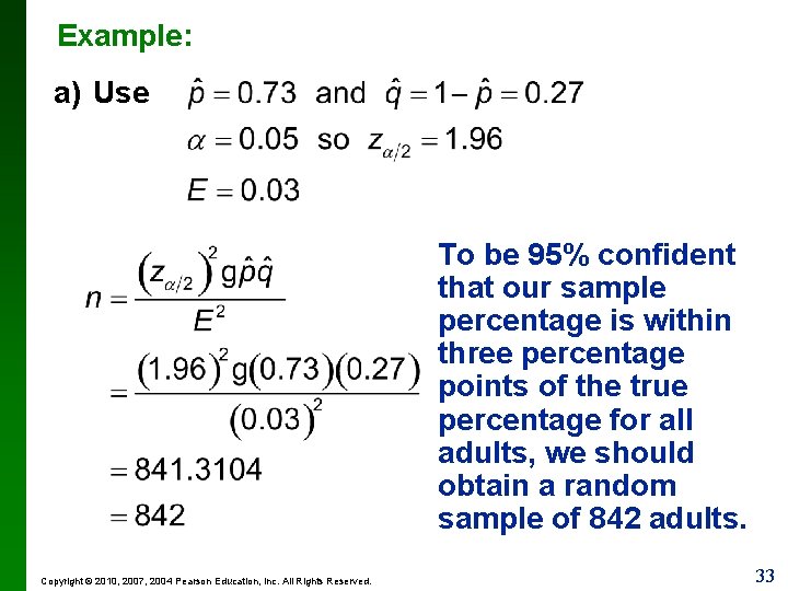
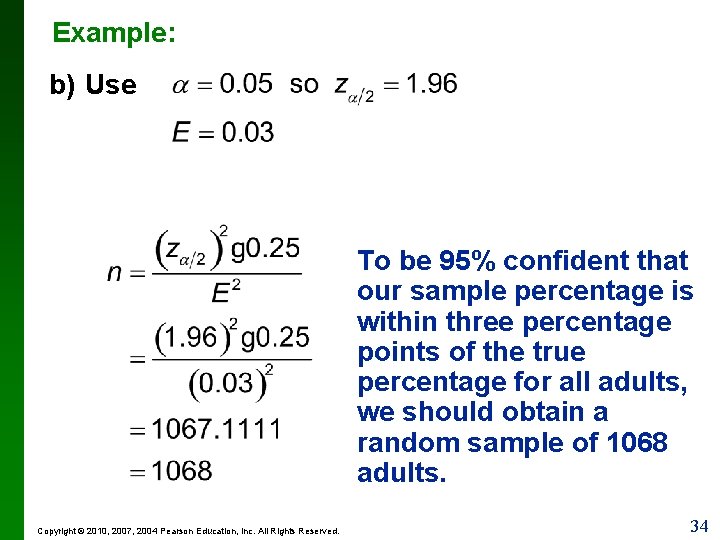
Example: A manager for E-Bay wants to determine the current percentage of U. S. adults who now use the Internet. How many adults must be surveyed in order to be 95% confident that the sample percentage is in error by no more than three percentage points? a) In 2006, 73% of adults used the Internet. b) No known possible value of the proportion. Copyright © 2010, 2007, 2004 Pearson Education, Inc. All Rights Reserved. 32

Example: a) Use To be 95% confident that our sample percentage is within three percentage points of the true percentage for all adults, we should obtain a random sample of 842 adults. Copyright © 2010, 2007, 2004 Pearson Education, Inc. All Rights Reserved. 33

Example: b) Use To be 95% confident that our sample percentage is within three percentage points of the true percentage for all adults, we should obtain a random sample of 1068 adults. Copyright © 2010, 2007, 2004 Pearson Education, Inc. All Rights Reserved. 34

Section 7. 3: Estimation of a population mean m ( is known) In this section we cover methods for estimating a population mean. In addition to knowing the values of the sample data or statistics, we must also know the value of the population standard deviation, . Copyright © 2010, 2007, 2004 Pearson Education, Inc. All Rights Reserved. 35

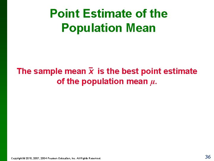
Point Estimate of the Population Mean The sample mean x is the best point estimate of the population mean µ. Copyright © 2010, 2007, 2004 Pearson Education, Inc. All Rights Reserved. 36

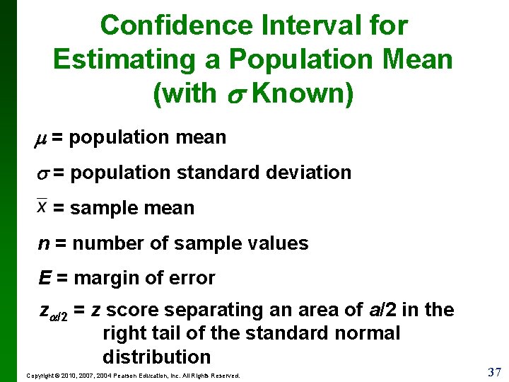
Confidence Interval for Estimating a Population Mean (with Known) = population mean = population standard deviation = sample mean n = number of sample values E = margin of error z /2 = z score separating an area of a/2 in the right tail of the standard normal distribution Copyright © 2010, 2007, 2004 Pearson Education, Inc. All Rights Reserved. 37

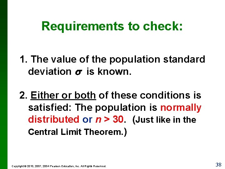
Requirements to check: 1. The value of the population standard deviation is known. 2. Either or both of these conditions is satisfied: The population is normally distributed or n > 30. (Just like in the Central Limit Theorem. ) Copyright © 2010, 2007, 2004 Pearson Education, Inc. All Rights Reserved. 38

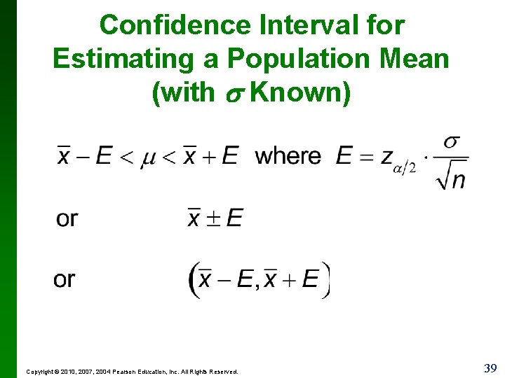
Confidence Interval for Estimating a Population Mean (with Known) Copyright © 2010, 2007, 2004 Pearson Education, Inc. All Rights Reserved. 39

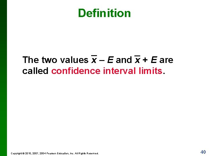
Definition The two values x – E and x + E are called confidence interval limits. Copyright © 2010, 2007, 2004 Pearson Education, Inc. All Rights Reserved. 40

Round-Off Rule for Confidence Intervals Used to Estimate µ 1. When using the original set of data, round the confidence interval limits to one more decimal place than used in original set of data. 2. When the original set of data is unknown and only the summary statistics (n, x, s) are used, round the confidence interval limits to the same number of decimal places used for the sample mean. Copyright © 2010, 2007, 2004 Pearson Education, Inc. All Rights Reserved. 41

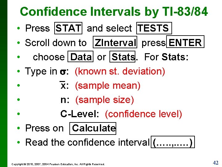
Confidence Intervals by TI-83/84 • • • Press STAT and select TESTS Scroll down to ZInterval press ENTER choose Data or Stats. For Stats: Type in : (known st. deviation) _ x: (sample mean) n: (sample size) C-Level: (confidence level) Press on Calculate Read the confidence interval (…. . , . . …) Copyright © 2010, 2007, 2004 Pearson Education, Inc. All Rights Reserved. 42

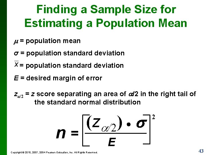
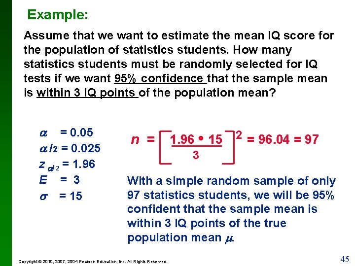
Finding a Sample Size for Estimating a Population Mean = population mean σ = population standard deviation E = desired margin of error zα/2 = z score separating an area of /2 in the right tail of the standard normal distribution n= (z /2) Copyright © 2010, 2007, 2004 Pearson Education, Inc. All Rights Reserved. E 2 43

Round-Off Rule for Sample Size n If the computed sample size n is not a whole number, round the value of n up to the next larger whole number. Copyright © 2010, 2007, 2004 Pearson Education, Inc. All Rights Reserved. 44

Example: Assume that we want to estimate the mean IQ score for the population of statistics students. How many statistics students must be randomly selected for IQ tests if we want 95% confidence that the sample mean is within 3 IQ points of the population mean? = 0. 05 /2 = 0. 025 z / 2 = 1. 96 E = 3 = 15 n = 1. 96 • 15 2 = 96. 04 = 97 3 With a simple random sample of only 97 statistics students, we will be 95% confident that the sample mean is within 3 IQ points of the true population mean . Copyright © 2010, 2007, 2004 Pearson Education, Inc. All Rights Reserved. 45

Section 7. 4: Estimation of a population mean m ( is not known) This section presents methods for estimating a population mean when the population standard deviation is not known. Copyright © 2010, 2007, 2004 Pearson Education, Inc. All Rights Reserved. 46

Sample Mean _ The sample mean x is still the best point estimate of the population mean m. Copyright © 2010, 2007, 2004 Pearson Education, Inc. All Rights Reserved. 47

Construction of a confidence intervals for m ( is not known) With σ unknown, we use the Student t distribution instead of normal distribution. It involves a new feature: number of degrees of freedom Copyright © 2010, 2007, 2004 Pearson Education, Inc. All Rights Reserved. 48

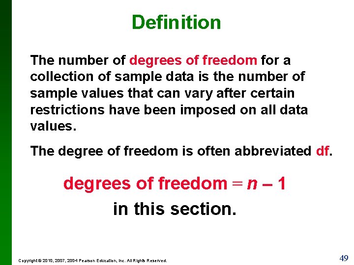
Definition The number of degrees of freedom for a collection of sample data is the number of sample values that can vary after certain restrictions have been imposed on all data values. The degree of freedom is often abbreviated df. degrees of freedom = n – 1 in this section. Copyright © 2010, 2007, 2004 Pearson Education, Inc. All Rights Reserved. 49

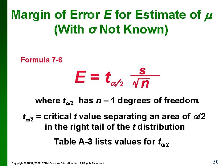
Margin of Error E for Estimate of (With σ Not Known) Formula 7 -6 E = t s 2 n where t /2 has n – 1 degrees of freedom. t /2 = critical t value separating an area of /2 in the right tail of the t distribution Table A-3 lists values for tα/2 Copyright © 2010, 2007, 2004 Pearson Education, Inc. All Rights Reserved. 50

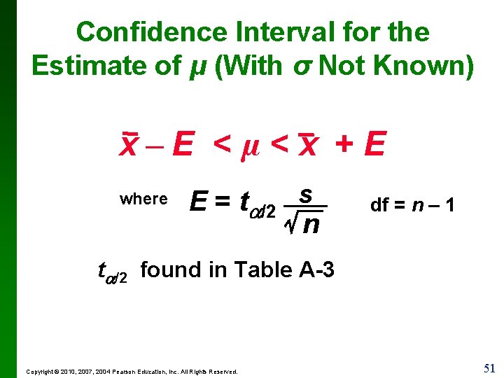
Confidence Interval for the Estimate of μ (With σ Not Known) x–E <µ<x +E where E = t /2 s n df = n – 1 t /2 found in Table A-3 Copyright © 2010, 2007, 2004 Pearson Education, Inc. All Rights Reserved. 51

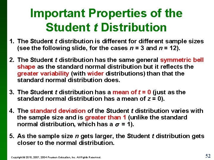
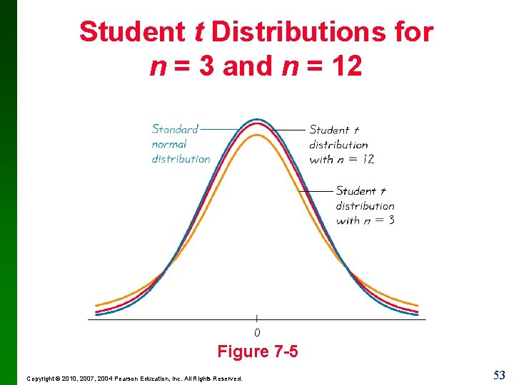
Important Properties of the Student t Distribution 1. The Student t distribution is different for different sample sizes (see the following slide, for the cases n = 3 and n = 12). 2. The Student t distribution has the same general symmetric bell shape as the standard normal distribution but it reflects the greater variability (with wider distributions) than that the standard normal distribution does. 3. The Student t distribution has a mean of t = 0 (just as the standard normal distribution has a mean of z = 0). 4. The standard deviation of the Student t distribution varies with the sample size and is greater than 1 (unlike the standard normal distribution, which has a = 1). 5. As the sample size n gets larger, the Student t distribution gets closer to the normal distribution. Copyright © 2010, 2007, 2004 Pearson Education, Inc. All Rights Reserved. 52

Student t Distributions for n = 3 and n = 12 Figure 7 -5 Copyright © 2010, 2007, 2004 Pearson Education, Inc. All Rights Reserved. 53

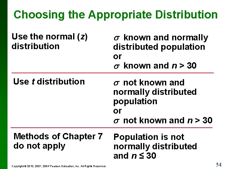
Choosing the Appropriate Distribution Use the normal (z) distribution Use t distribution known and normally distributed population or known and n > 30 not known and normally distributed population or not known and n > 30 Methods of Chapter 7 do not apply Copyright © 2010, 2007, 2004 Pearson Education, Inc. All Rights Reserved. Population is not normally distributed and n ≤ 30 54

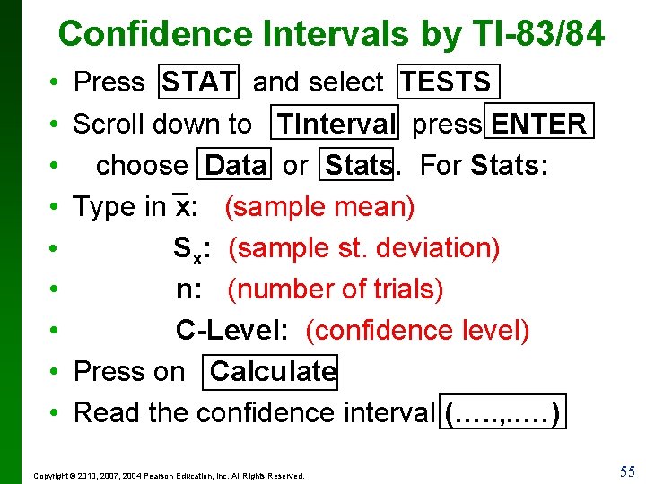
Confidence Intervals by TI-83/84 • • • Press STAT and select TESTS Scroll down to TInterval press ENTER choose Data or Stats. For Stats: _ Type in x: (sample mean) Sx: (sample st. deviation) n: (number of trials) C-Level: (confidence level) Press on Calculate Read the confidence interval (…. . , . . …) Copyright © 2010, 2007, 2004 Pearson Education, Inc. All Rights Reserved. 55

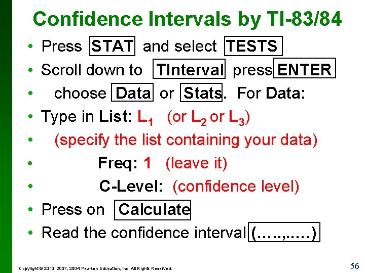
Confidence Intervals by TI-83/84 • • • Press STAT and select TESTS Scroll down to TInterval press ENTER choose Data or Stats. For Data: Type in List: L 1 (or L 2 or L 3) (specify the list containing your data) Freq: 1 (leave it) C-Level: (confidence level) Press on Calculate Read the confidence interval (…. . , . . …) Copyright © 2010, 2007, 2004 Pearson Education, Inc. All Rights Reserved. 56

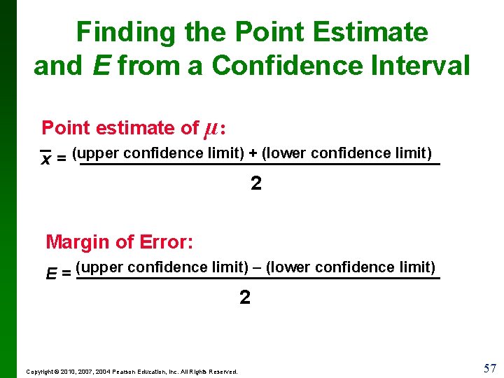
Finding the Point Estimate and E from a Confidence Interval Point estimate of µ: x = (upper confidence limit) + (lower confidence limit) 2 Margin of Error: E = (upper confidence limit) – (lower confidence limit) 2 Copyright © 2010, 2007, 2004 Pearson Education, Inc. All Rights Reserved. 57

Section 7 -5 Estimating a Population Variance This section covers the estimation 2 of a population variance and standard deviation . Copyright © 2010, 2007, 2004 Pearson Education, Inc. All Rights Reserved. 58

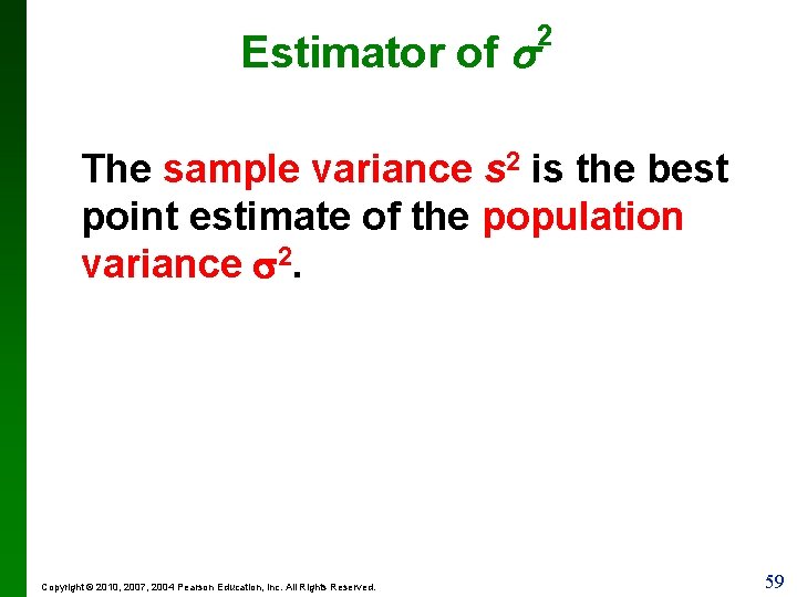
Estimator of 2 The sample variance s 2 is the best point estimate of the population variance 2. Copyright © 2010, 2007, 2004 Pearson Education, Inc. All Rights Reserved. 59

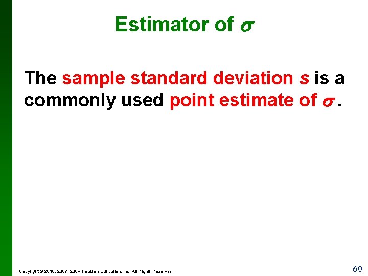
Estimator of The sample standard deviation s is a commonly used point estimate of . Copyright © 2010, 2007, 2004 Pearson Education, Inc. All Rights Reserved. 60

Construction of confidence 2 intervals for We use the chi-square distribution, denoted by Greek character 2 (pronounced chi-square). Copyright © 2010, 2007, 2004 Pearson Education, Inc. All Rights Reserved. 61

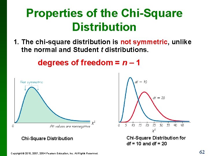
Properties of the Chi-Square Distribution 1. The chi-square distribution is not symmetric, unlike the normal and Student t distributions. degrees of freedom = n – 1 Chi-Square Distribution Copyright © 2010, 2007, 2004 Pearson Education, Inc. All Rights Reserved. Chi-Square Distribution for df = 10 and df = 20 62

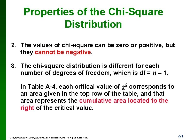
Properties of the Chi-Square Distribution 2. The values of chi-square can be zero or positive, but they cannot be negative. 3. The chi-square distribution is different for each number of degrees of freedom, which is df = n – 1. In Table A-4, each critical value of 2 corresponds to an area given in the top row of the table, and that area represents the cumulative area located to the right of the critical value. Copyright © 2010, 2007, 2004 Pearson Education, Inc. All Rights Reserved. 63

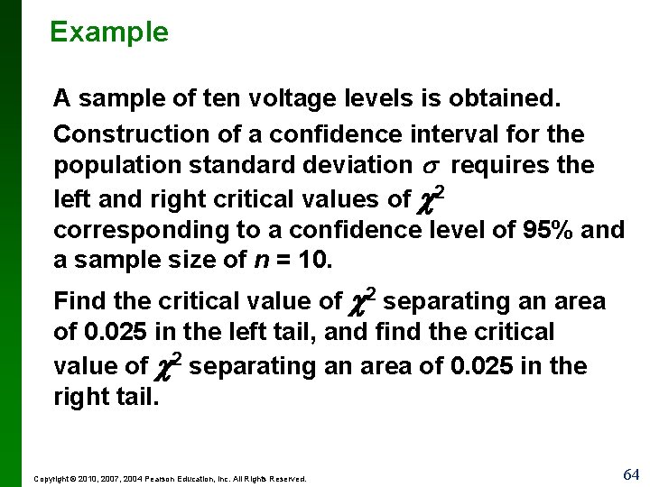
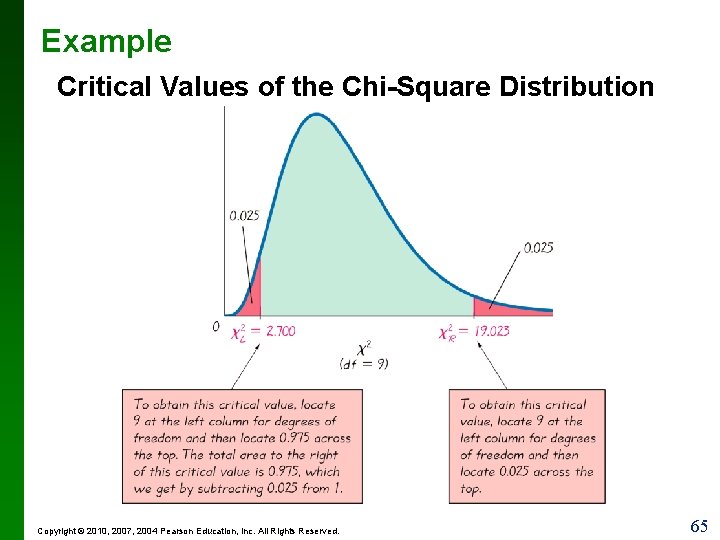
Example A sample of ten voltage levels is obtained. Construction of a confidence interval for the population standard deviation requires the left and right critical values of 2 corresponding to a confidence level of 95% and a sample size of n = 10. Find the critical value of 2 separating an area of 0. 025 in the left tail, and find the critical value of 2 separating an area of 0. 025 in the right tail. Copyright © 2010, 2007, 2004 Pearson Education, Inc. All Rights Reserved. 64

Example Critical Values of the Chi-Square Distribution Copyright © 2010, 2007, 2004 Pearson Education, Inc. All Rights Reserved. 65

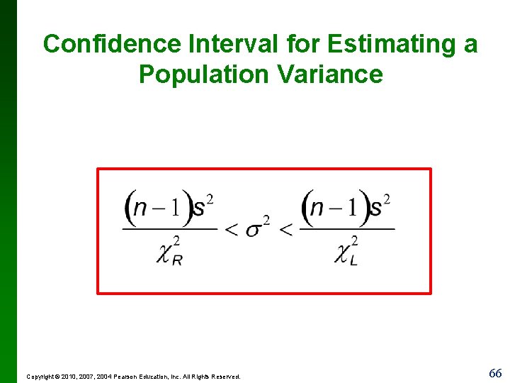
Confidence Interval for Estimating a Population Variance Copyright © 2010, 2007, 2004 Pearson Education, Inc. All Rights Reserved. 66

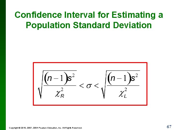
Confidence Interval for Estimating a Population Standard Deviation Copyright © 2010, 2007, 2004 Pearson Education, Inc. All Rights Reserved. 67

Requirement: The population must have normally distributed values (even if the sample is large) This requirement is very strict Copyright © 2010, 2007, 2004 Pearson Education, Inc. All Rights Reserved. 68

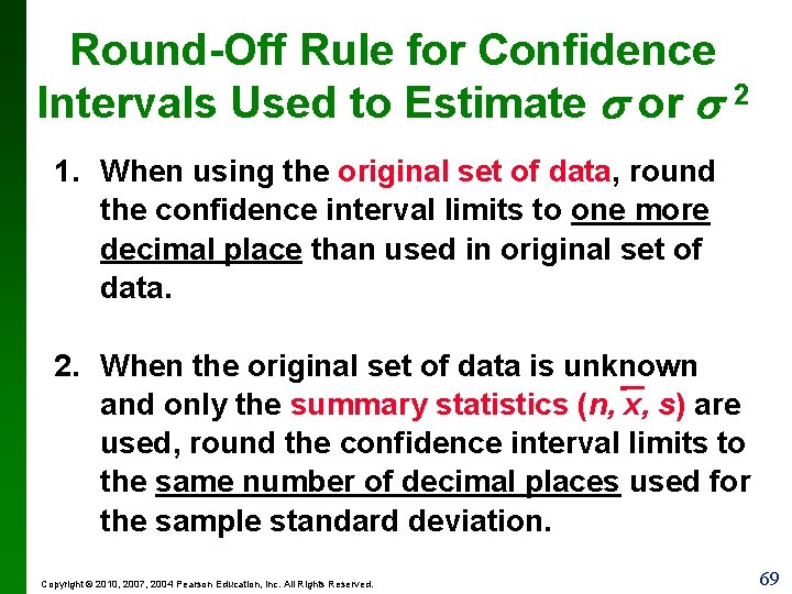
Round-Off Rule for Confidence Intervals Used to Estimate or 2 1. When using the original set of data, round the confidence interval limits to one more decimal place than used in original set of data. 2. When the original set of data is unknown and only the summary statistics (n, x, s) are used, round the confidence interval limits to the same number of decimal places used for the sample standard deviation. Copyright © 2010, 2007, 2004 Pearson Education, Inc. All Rights Reserved. 69

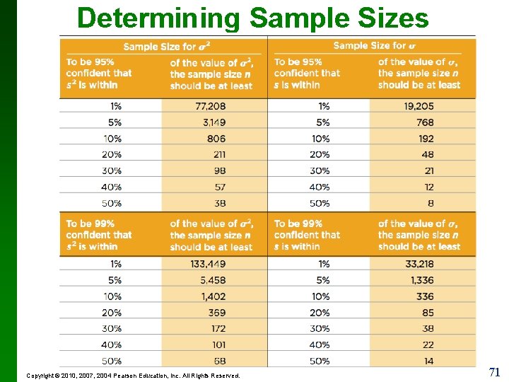
Determining Sample Sizes The procedure for finding the sample size necessary to estimate 2 is based on Table 7 -2. You just read the required sample size from an appropriate line of the table. Copyright © 2010, 2007, 2004 Pearson Education, Inc. All Rights Reserved. 70

Determining Sample Sizes Copyright © 2010, 2007, 2004 Pearson Education, Inc. All Rights Reserved. 71

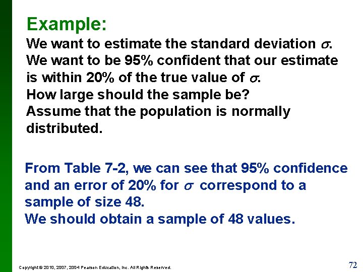
Example: We want to estimate the standard deviation . We want to be 95% confident that our estimate is within 20% of the true value of . How large should the sample be? Assume that the population is normally distributed. From Table 7 -2, we can see that 95% confidence and an error of 20% for correspond to a sample of size 48. We should obtain a sample of 48 values. Copyright © 2010, 2007, 2004 Pearson Education, Inc. All Rights Reserved. 72