Example A student attempts a multiple choice exam

Example A student attempts a multiple choice exam (options A to F for each question), but having done no work, selects his answers to each question by rolling a fair die (A = 1, B = 2, etc. ). If the exam contains 100 questions, what is the probability of obtaining a mark below 20?

Simulation Now, let us simulate a large number of realisations of students using this random method of answering multiple choice questions. We still require the same Binomial distribution with n=100 and a= This can be done on R using the command rbinom.

For example, let’s simulate 1000 students. > xsim=rbinom(1000, 1/6) > xsim [1] 18 22 9 17 18 20 21 16 8 18 11 16 16 13 16 14 25 15 16 17 [21] 13 25 11 24 17 16 13 21 10 17 18 19 17 19 15 13 12 [41] 15 11 21 23 19 14 19 25 23 19 20 17 17 15 16 14 13 16 17 14 [61] 24 21 19 8 18 20 22 16 15 20 19 17 13 15 13 21 22 12 12 12 [81] 11 14 11 12 16 16 17 21 17 16 17 14 9 17 16 17 12 20 16 17 [101] 18 13 15 16 12 15 17 16 17 26 18 14 21 15 10 23 12 16 16 12 [121] 17 18 22 17 18 14 19 22 13 17 21 15 21 16 17 16 16 28 16 17 [141] 18 19 16 11 14 18 16 18 18 14 20 13 19 19 22 22 13 17 19 17 [161] 18 20 11 22 19 25 15 15 17 18 5 15 14 13 18 15 17 15 20 17 [181] 16 14 23 17 16 10 12 16 21 30 16 13 22 14 15 16 17 14 16 18 [201] 14 20 16 19 25 14 15 24 22 19 15 17 22 10 20 13 10 15 14 22 [221] 17 12 16 19 20 17 15 21 14 13 21 11 19 9 21 22 16 13 13 12 [241] 14 13 18 8 14 18 10 16 10 12 21 18 15 17 16 8 19 17 11 18 [261] 23 17 20 16 12 20 11 16 22 17 16 13 22 20 15 15 20 17 22 14 [281] 18 23 18 20 20 16 19 16 15 19 18 17 14 22 15 24 17 15 17 22

[301] 18 22 10 19 24 21 16 14 11 14 20 15 21 11 17 16 20 19 13 14 [321] 17 17 19 15 17 13 18 23 16 12 25 13 13 21 19 16 20 27 19 18 [341] 18 24 15 23 13 13 14 15 23 13 19 15 11 19 17 12 15 15 17 14 [361] 18 20 17 13 16 14 13 20 18 15 18 16 17 20 14 19 21 12 13 17 [381] 22 17 19 16 14 18 16 18 12 16 13 15 16 9 15 16 18 22 14 16 [401] 14 17 12 16 21 13 14 19 18 18 16 19 17 17 17 13 17 11 [421] 16 16 13 10 26 12 20 17 11 19 18 12 15 14 14 20 15 15 15 11 [441] 18 23 20 23 13 12 18 22 12 16 13 21 22 14 18 21 17 12 19 16 [461] 17 18 15 22 22 20 15 16 13 12 19 22 16 20 19 19 16 8 15 12 [481] 29 26 19 16 20 15 11 22 15 20 21 14 16 13 17 15 10 13 17 12 [501] 18 20 17 14 13 19 23 11 27 19 17 16 17 20 21 15 20 20 21 19 [521] 21 16 13 21 16 19 13 9 10 20 12 18 14 13 18 19 22 19 21 18 [541] 6 17 17 19 19 22 23 18 13 12 17 16 21 16 18 21 19 13 22 19 [561] 20 17 18 15 17 15 15 10 18 13 23 17 14 23 22 10 18 11 11 18 [581] 16 17 14 13 9 12 14 14 21 23 24 19 12 15 17 18 11 14 19 19 [601] 19 16 17 13 13 15 17 18 17 13 9 19 18 22 17 13 14 22 13 23 [621] 23 19 19 16 24 14 17 18 17 13 16 12 7 15 17 16 18 22 19 15 [641] 16 18 18 13 20 18 12 6 15 11 16 19 12 13 11 17 11 15 11 19

[661] 17 16 16 21 12 18 20 19 16 14 18 17 16 14 11 17 17 16 17 17 [681] 17 18 16 18 12 18 18 20 19 13 12 16 14 13 13 6 15 12 19 14 [701] 20 17 16 14 21 19 15 26 17 20 12 24 13 11 19 21 18 13 9 16 [721] 9 16 17 16 15 12 11 21 21 13 19 13 13 16 11 17 15 19 22 19 [741] 11 13 14 16 20 15 16 12 18 14 12 14 21 12 23 21 19 10 24 17 [761] 17 19 19 15 18 12 14 14 14 20 12 21 19 20 21 20 17 18 [781] 15 12 16 23 16 16 19 15 12 14 21 25 12 19 20 22 17 16 21 20 [801] 23 24 17 20 17 19 14 22 20 25 10 12 15 16 7 14 14 18 22 10 [821] 15 22 23 18 12 10 14 18 15 15 18 10 21 11 20 15 20 10 13 16 [841] 16 17 22 19 19 16 8 20 17 13 21 16 25 16 13 17 14 17 19 21 [861] 17 19 14 22 20 18 14 19 17 23 20 18 14 11 16 18 26 24 24 18 [881] 21 16 23 20 14 16 15 13 14 11 12 13 14 16 18 17 16 17 13 20 [901] 22 8 17 17 16 16 14 22 17 18 18 21 15 11 20 21 18 15 19 21 [921] 16 22 14 12 16 20 16 21 11 13 19 14 23 12 12 17 14 15 26 17 [941] 18 14 21 17 14 24 21 12 21 13 20 22 11 20 10 16 16 15 19 13 [961] 16 15 16 17 9 14 11 12 19 17 16 15 21 14 15 17 15 16 [981] 19 11 15 17 17 17 11 18 21 14 15 17 18 16 11 22 19 16 14 15

It makes sense now to look at properties of these 1000 simulations which have been placed in the vector “xsim”. > mean(xsim) [1] 16. 624 > median(xsim) [1] 17 > sd(xsim) [1] 3. 778479 > var(xsim) [1] 14. 2769 >

Now compare the actual values from the simulations, with theoretical values from the probability distribution. SIMULATION THEORETICAL MEAN 16. 624 16. 66667 VARIANCE 14. 2769 13. 88889

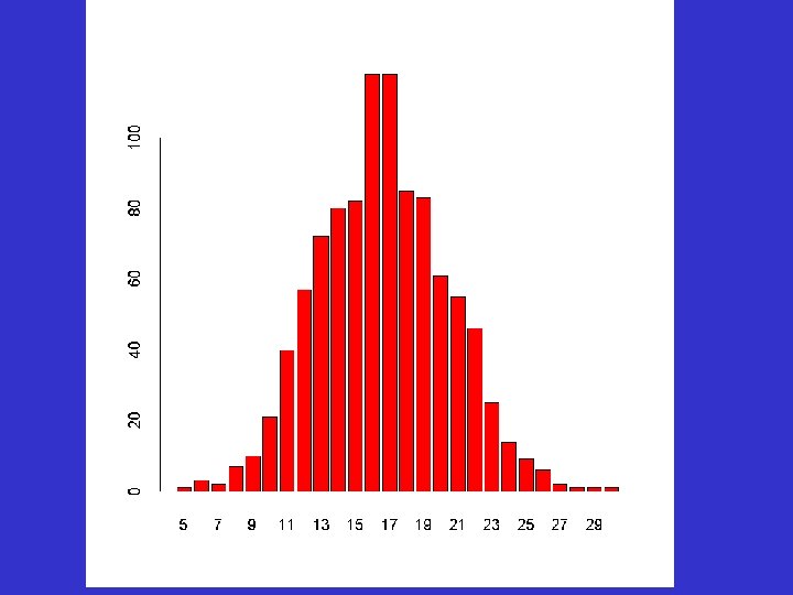
A full summary of the results of the simulation is given with: > table(xsim) xsim 5 6 7 8 9 10 11 12 13 14 15 16 17 1 3 2 7 10 21 40 57 72 80 82 118 18 19 20 21 22 23 24 25 26 27 28 29 30 85 83 61 55 46 25 14 9 6 2 1 1 1 >

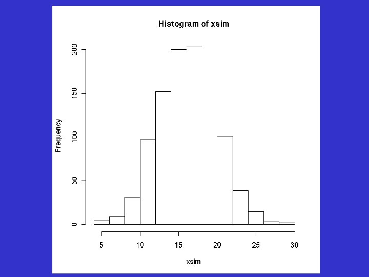
A Histogram can also be plotted of this: > hist(xsim)

Notice that a BARPLOT of xsim does NOT produce a useful graph! > barplot(xsim)

A barplot of the TABLE of xsim does work, though. > barplot(table(xsim))

Poisson Distribution The Poisson distribution is used to model the number of events occurring within a given time interval. The formula for the Poisson probability density (mass) function is the shape parameter which indicates the average number of events in the given time interval.

Some events are rather rare - they don't happen that often. For instance, car accidents are the exception rather than the rule. Still, over a period of time, we can say something about the nature of rare events. An example is the improvement of traffic safety, where the government wants to know whether seat belts reduce the number of death in car accidents. Here, the Poisson distribution can be a useful tool to answer questions about benefits of seat belt use.

Other phenomena that often follow a Poisson distribution are death of infants, the number of misprints in a book, the number of customers arriving, and the number of activations of a Geiger counter. The distribution was derived by the French mathematician Siméon Poisson in 1837, and the first application was the description of the number of deaths by horse kicking in the Prussian army.

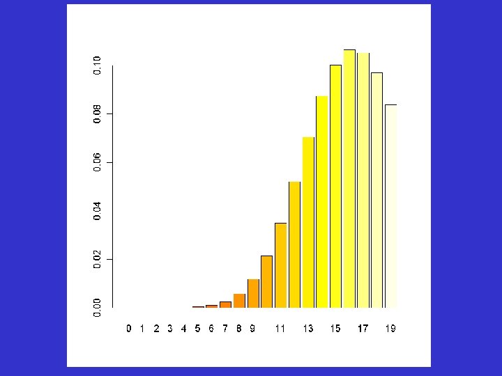
Example Arrivals at a bus-stop follow a Poisson distribution with an average of 4. 5 every quarter of an hour. Obtain a barplot of the distribution (assume a maximum of 20 arrivals in a quarter of an hour) and calculate the probability of fewer than 3 arrivals in a quarter of an hour.

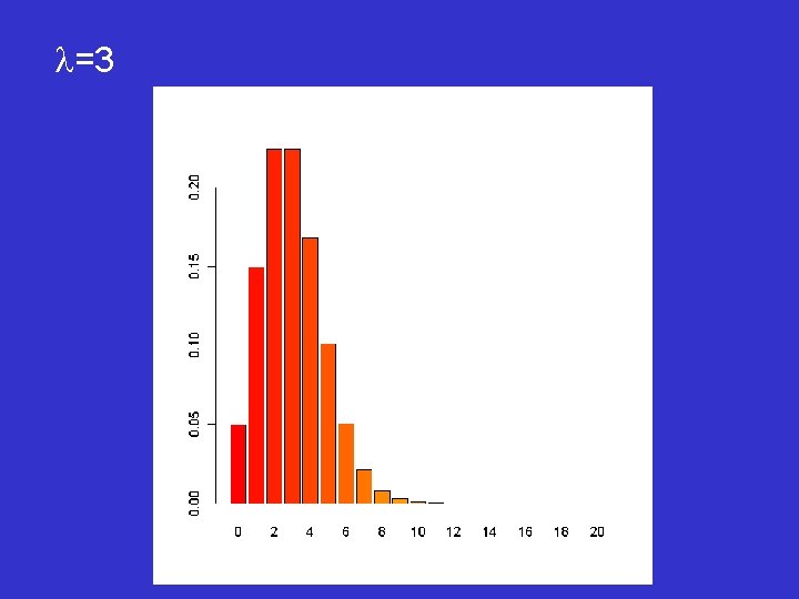
The probabilities of 0 up to 2 arrivals can be calculated directly from the formula with =4. 5 So p(0) = 0. 01111

Similarly p(1)=0. 04999 and p(2)=0. 11248 So the probability of fewer than 3 arrivals is 0. 01111+ 0. 04999 + 0. 11248 =0. 17358

R Code As with the Binomial distribution, the codes dpois and ppois will do the calculations for you.

> x=dpois(0: 20, 4. 5) >x [1] 1. 110900 e-02 4. 999048 e-02 1. 124786 e-01 1. 687179 e-01 1. 898076 e-01 [6] 1. 708269 e-01 1. 281201 e-01 8. 236295 e-02 4. 632916 e-02 2. 316458 e-02 [11] 1. 042406 e-02 4. 264389 e-03 1. 599146 e-03 5. 535504 e-04 1. 779269 e-04 [16] 5. 337808 e-05 1. 501258 e-05 3. 973919 e-06 9. 934798 e-07 2. 352979 e-07 [21] 5. 294202 e-08 >

> barplot(x, names=0: 20)

Now check that ppois gives the same answer (ppois is a cumulative distribution). > ppois(2, 4. 5) [1] 0. 1735781 >

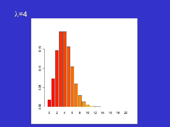
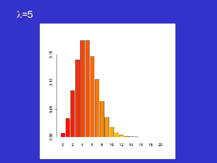
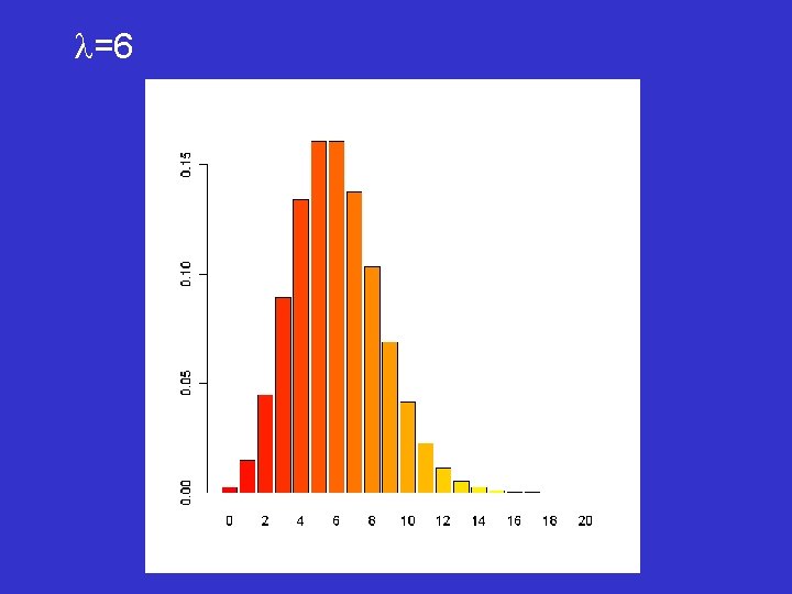
Consider a collection of graphs for different values of

=10

In the last case, the probability of 20 arrivals is no longer negligible, so values up to, say, 30 would have to be considered.

Properties of Poisson The mean and variance are both equal to . The sum of independent Poisson variables is a further Poisson variable with mean equal to the sum of the individual means. As well as cropping up in the situations already mentioned, the Poisson distribution provides an approximation for the Binomial distribution.

Approximation: If n is large and p is small, then the Binomial distribution with parameters n and p, ( B(n; p) ), is well approximated by the Poisson distribution with parameter np, i. e. by the Poisson distribution with the same mean

Example Binomial situation, n= 100, p=0. 075 Calculate the probability of fewer than 10 successes.

> pbinom(9, 100, 0. 075) [1] 0. 7832687 > This would have been very tricky with manual calculation as the factorials are very large and the probabilities very small

The Poisson approximation to the Binomial states that will be equal to np, i. e. 100 x 0. 075 so =7. 5 > ppois(9, 7. 5) [1] 0. 7764076 > So it is correct to 2 decimal places. Manually, this would have been much simpler to do than the Binomial.