Example 6 4 Plant and Warehouse Location Models

Example 6. 4 Plant and Warehouse Location Models

Background Information n Huntco produces tomato sauce at five different plants. n The capacity (in tons) of each plant is given in the following table. Capacities for Huntco Example Plant Tons 1 2 3 4 5 300 200 400 6. 1 | 6. 2 | 6. 3 | 6. 5 | 6. 6 | 6. 7

Background Information -continued n The tomato sauce is stored at one of three warehouses. The cost per ton of producing tomato sauce at each plant and shipping it to each warehouse is given in the table shown here. Production and Shipping Costs for Huntco Example To From Warehouse 1 Warehouse 2 Warehouse 3 Plant 1 $800 $1000 $1200 Plant 2 $700 $500 $700 Plant 3 $800 $600 $500 Plant 4 $500 $600 $700 Plant 5 $700 $600 $500 6. 1 | 6. 2 | 6. 3 | 6. 5 | 6. 6 | 6. 7

Background Information -continued n Huntco has four customers. n The cost of shipping a ton of sauce from each warehouse to each customer is given in the table shown here. Shipping Costs to Customers for Huntco Example To From Customer 1 Customer 2 Customer 3 Customer 4 Warehouse 1 $40 $80 $90 $50 Warehouse 2 $70 $40 $60 $80 Warehouse 3 $80 $30 $50 $60 6. 1 | 6. 2 | 6. 3 | 6. 5 | 6. 6 | 6. 7

Background Information -continued n Each customer must receive the amount (in tons) of sauce given in the following table. Customer Requirements for Huntco Example Customer Requirements 1 2 3 4 200 300 150 250 6. 1 | 6. 2 | 6. 3 | 6. 5 | 6. 6 | 6. 7

Background Information -continued n The annual fixed cost of operating each plant and warehouse is listed in this table. Fixed Costs for Huntco Example Fixed Annual Cost Plant 1 $35, 000 Plant 2 $45, 000 Plant 3 $40, 000 Plant 4 $42, 000 Plant 5 $40, 000 Warehouse 1 $40, 000 Warehouse 2 $20, 000 Warehouse 3 $60, 000 6. 1 | 6. 2 | 6. 3 | 6. 5 | 6. 6 | 6. 7

Background Information -continued n Huntco’s goal is to minimize the annual cost of meeting customer demands. n The company wants to determine which plants and warehouses to open, as well as the optimal shipping plan. 6. 1 | 6. 2 | 6. 3 | 6. 5 | 6. 6 | 6. 7

Solution n To model Huntco’s situation we need to keep track of the following: – The shipments from plants to warehouses – The shipments from warehouses to customers – The fixed costs of operating plants and warehouses – The shipping and production costs from plants to warehouses – The shipping costs from warehouses to customers – The total amount shipped out of each plant 6. 1 | 6. 2 | 6. 3 | 6. 5 | 6. 6 | 6. 7

Solution -- continued n We must also ensure that – Huntco pays the fixed costs for all plants and warehouses that it uses. – The amount shipped into each warehouse equals the amount received by each warehouse. – Each customer receives the specified demand. 6. 1 | 6. 2 | 6. 3 | 6. 5 | 6. 6 | 6. 7

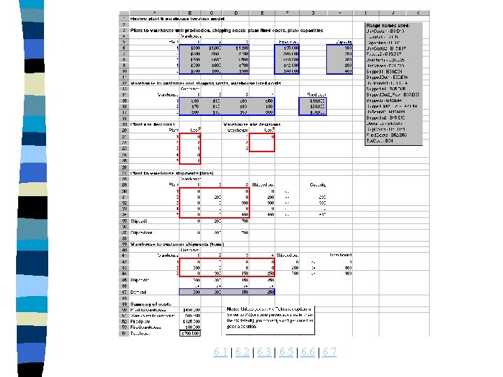
HUNTCO. XLS n The spreadsheet model is shown on the next slide. n This file can be used to complete the model. 6. 1 | 6. 2 | 6. 3 | 6. 5 | 6. 6 | 6. 7

Developing the Model n To form the model, follow these steps: – Inputs. Enter the given data in the shaded ranges. – Shipments. Enter any trial values for the shipments from each plant to each warehouse in the Shipped 1 range and any trial values for the shipments from each warehouse to each customer in the Shipped 2 range. – Binary fixed cost variables. Enter any trial 0 -1 values for the plant fixed-cost variables in the Use. Plants range and the warehouse fixed-cost variables in the Use. Whses range. The fixed-cost variable for a plant equals 1 if the plant is used and 0 if the plant is not used. Similarly, the fixed-cost variable for a warehouse equals 1 if the warehouse is used and 0 if the warehouse is not used. 6. 1 | 6. 2 | 6. 3 | 6. 5 | 6. 6 | 6. 7

Developing the Model -continued – Amount shipped out of each plant. Calculate the amounts shipped out of the plants as row sums in the Shipped. Out 1 range. Specifically, enter the formula =SUM(B 30: D 30) in cell E 30 and copy it to the rest of the Shipped. Out 1 range. – Upper limit on amount shipped out of each plant. For each plant we need a constraint of the form Total shipped out of plant Plant capacity * Fixed-cost variable for plant This inequality ensures that if Huntco uses the plant, then this plant’s fixed-cost variable will equal 1 and the company will have to pay the plant’s operating cost. In this case the inequality states that the total shipped out of the plant is less than or equal to the plant’s capacity. 6. 1 | 6. 2 | 6. 3 | 6. 5 | 6. 6 | 6. 7

Developing the Model -continued – We generate the right side of the inequality in the Up. Counds 1 range. Specifically, enter the formula =B 21*H 6 in cell G 30 and copy it to the rest of the Up. Bounds 1 range. Note that if a plant is not used, the Solver is free to make this plant’s fixed-cost variable 0, and no fixed cost for this plant will be incurred. Then the inequality will be satisfied trivially (0 0). – Amount shipped into and out of each warehouse. For each warehouse, we need “flow balance” – that is, we need the following constraint: Total shipments into warehouse = Total shipments out of warehouse To implement this equation, first calculate the left side as column sums in the Shipped. In 1 range. That is, enter the formula =SUM(B 30: B 34) in cell B 35 and copy it to the rest of the Shipped. In 1 range. 6. 1 | 6. 2 | 6. 3 | 6. 5 | 6. 6 | 6. 7

Developing the Model -continued – For the right side of the equality, first calculate total shipments out of warehouses as row sums in the Shipped. Out 2_Col column range. That is enter the formula =SUM(B 42: E 42) in cell F 42 and copying it to the rest of the Shipped. Out 2_Col range, entering the formula totals in the Shipped. Out 2_Row range by selecting this range, entering the formula =TRANSPOSE(Shipped. Out 2_Col) and pressing Ctrl-Shift-Enter. This allows us to compare a row with a row when we specify the equation in the Solver dialog box. – Upper limit on amount shipped out of each warehouse. For each warehouse we need a constraint of the form Total shipped out of warehouse Upper. Bound * Fixed-cost variable for warehouse 6. 1 | 6. 2 | 6. 3 | 6. 5 | 6. 6 | 6. 7

Developing the Model -continued – Here Upper. Bound is an upper bound on the most that could possibly be shipped out of any warehouse. Several possibilities for Upper. Bound could be used. We use the smaller of the total demand for all customers and the total capacity for all plants. If a warehouse’s fixed-cost variable is 0, then the inequality ensures that this warehouse cannot be used, whereas if the fixed-cost variable is 1, then this inequality is satisfied automatically. To operationalize the inequality, note that we already have the left sides in the Shipped. Out 2_Col range. To calculate the right side, enter the formula =E 21*MIN(SUM(Capacities), (SUM(Demands)) in cell H 42 and copy it to the rest of the Up. Bounds 2 range. 6. 1 | 6. 2 | 6. 3 | 6. 5 | 6. 6 | 6. 7

Developing the Model -continued – Amount received by each customer. Calculate the total amounts received by the customers as column sums in the Shipped. In 2 range. That is, enter the formula =SUM(B 42: B 44) in cell B 45 and copy it to the rest of the Shipped. In 2 range. – Shipping costs. Calculate the total costs of shipping from plants to warehouses and from warehouses to customers in cells B 50 and B 51 with the formulas =SUMPRODUCT(Unit. Costs 1, Shipped 1) and =SUMPRODUCT(Unit. Costs 2, Shipped 2). – Fixed costs. Calculate the annual fixed costs for operating plants and warehouses in cells B 52 and B 53 with the formulas =SUMPRODUCT(FCosts 1, Use. Plants) and =SUMPRODUCT(FCosts 2, Use. Whses). 6. 1 | 6. 2 | 6. 3 | 6. 5 | 6. 6 | 6. 7

Developing the Model -continued – Total cost. Finally, calculate the total annual cost in the Tot. Cost cell with the formula =SUM(Ship. Costs, Fixed. Costs). 6. 1 | 6. 2 | 6. 3 | 6. 5 | 6. 6 | 6. 7

Using the Solver n The completed Solver dialog box is shown here. 6. 1 | 6. 2 | 6. 3 | 6. 5 | 6. 6 | 6. 7

Using the Solver -- continued n The following is the explanation of the setup of the previous dialog box. – Objective. The objective to minimize is total annual cost. – Changing cells. There are four sets of changing cells – two sets for amounts to ship and two sets of binary variables for which plants and warehouses to use. – Plant upper bounds. The constraint Shipped. Out 1<=Up. Bounds 1 operationalizes the first inequality. – Warehouse upper bounds. The constraint Shipped. Out 2_Col<=Up. Bounds 2 operationalizes the second inequality. 6. 1 | 6. 2 | 6. 3 | 6. 5 | 6. 6 | 6. 7

Using the Solver -- continued – Warehouse balance. The constraint Shipped. In 1=Shipped. Out 2_Row operationalizes the equality. – Demand constraints. The constraint Shipped. In 2>=Demands ensures that each customer received the required amount. 6. 1 | 6. 2 | 6. 3 | 6. 5 | 6. 6 | 6. 7

Solution n The optimal solution shown indicates that Huntco should use plants 2, 3, and 5 and warehouses 2 and 3. n Of course, the optimal shipping plan, as specified in the Shipped 1 and Shipped 2 ranges, uses only these plants and warehouses. n This solution incurs a total annual cost of $700, 500. n If you obtain an “optimal” solution with a total cost somewhat larger than this, check the Solver tolerance setting. If it is at its default level of 5%, the Solver might very well stop short of optimal. We obtained our solution by setting the tolerance to 0%. 6. 1 | 6. 2 | 6. 3 | 6. 5 | 6. 6 | 6. 7

Solution -- continued n At this point, you might want to review the inputs for this problem and see whether the optimal solution appears reasonable from an economic point of view. n For example, although plant 1 has a relatively small fixed cost, it has relatively large unit shipping costs. n This is evidently the reason for not using plant 1. n However, the situation is not so obvious for plant 4 or warehouse 1. We think you will agree that on logistics problems such as this – and this is not even a large problem – more than intuition is necessary! 6. 1 | 6. 2 | 6. 3 | 6. 5 | 6. 6 | 6. 7

Sensitivity Analysis n We will not report any specific sensitivity analyses for this model, but many are possible. n For example, we might check whether adding larger capacities at plants 1 and 4 would induce Huntco to open them. n Or we might see what would happen if all the fixed costs increases by some percentage. n Or we might see what would happen if all customer demands increased by some percentage. n Solver. Table, after some slight model modifications, can easily analyze any of these situations. 6. 1 | 6. 2 | 6. 3 | 6. 5 | 6. 6 | 6. 7