Example 1 A single looped network is shown

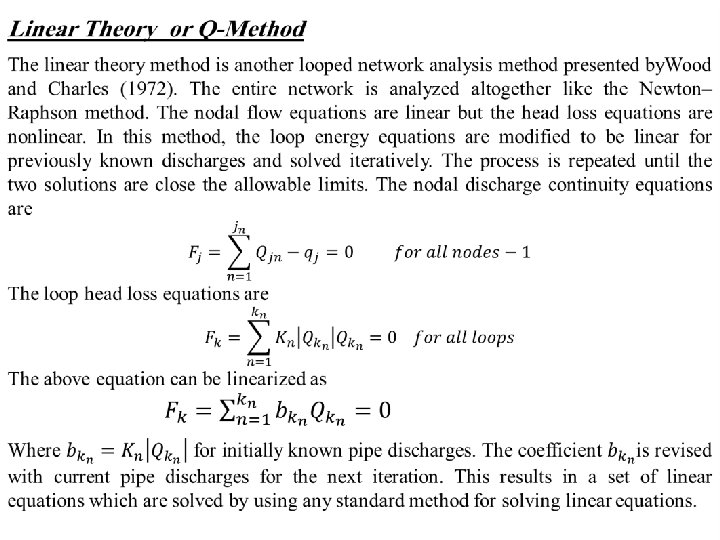
Example 1: A single looped network is shown below. Calculate the discharges in pipes by using Linear method. Solution

All details of the solution are explained in the following table

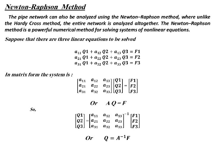
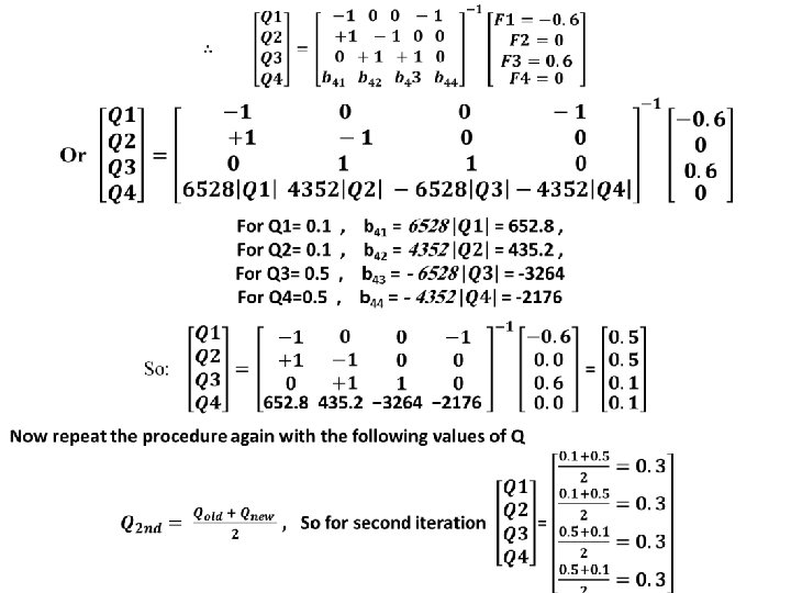
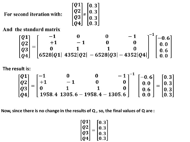
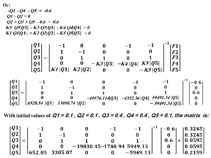
Example 2: The pipe network of two loops as shown in below has to be analyzed by Newton Raphson method for pipe flows for given pipe lengths L and pipe diameters D. The nodal inflow at node 1 and nodal outflow at node 3 are shown in the figure. Assume a constant friction factor f = 0. 02. Solution To apply continuity equation for initial pipe discharges, the discharges in pipes 1 and 5 equal to 0. 1 m 3/s are assumed. The obtained discharges are Q 1 = 0. 1 m 3/s Q 2 = 0. 1 m 3/s Q 3 = 0. 4 m 3/s Q 4 = 0. 4 m 3/s Q 5 = 0. 1 m 3/s

All details of the solution are explained in the following table

Example 3: For the piping system shown below, determine the flow distribution and piezometric heads at the junctions using the Linear Method.

All details of the solution are explained in the following table

Example 4: Re solve example 3 considering a pump located at pipe 1 with Hp = 250 – 0. 4 Q – 0. 1 Q 2

All details of the solution are explained in the following table

Note that for Q 5= - 0. 26135, it means that the flow must be in the opposite direction

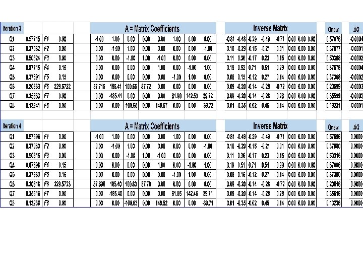
Note that with the following initial values of Q 1 = 0. 9 , Q 2 = 0. 4 , Q 3 = 0. 3, Q 4 = 0. 6 , Q 5 = 0. 3, Q 6= 0. 5 , Q 7= 0. 35 & Q 8= 0. 1 the solution will be as follows

All details of the solution are explained in the following table

Example 5: Re solve example 3 considering a pump located at pipe 4 with Hp = 250 – 0. 4 Q – 0. 1 Q 2

All details of the solution are explained in the following table

Example 6: For the piping system shown below, determine the flow distribution and piezometric heads at the junction J using Linear method of solution Solution [1] [2] Assuming initial pipe discharge in pipes, Q 1 = 0. 2 , Q 2 = 0. 2 & Q 3 = 0. 4. D (m) Pipe L (m) f 1 1500 0. 3 0. 01 0 2 1500 0. 3 0. 01 0 3 1500 0. 3 0. 01 0

All details of the solution are explained in the following table Note that for Q 2= - 0. 0795, it means that the flow must be in the opposite direction

Example 7: For the piping system shown below, determine the flow distribution and piezometric heads at the junction J using Linear method. Power = 20 Kw Solution [1] [2] Assuming initial pipe discharge in pipes, Q 1 = 0. 05 , Q 2 = 0. 05 & Q 3 = 0. 1. Pipe L (m) D (m) f 1 50 0. 15 0. 02 2 2 100 0. 10 0. 015 1 3 300 0. 10 0. 025 1

All details of the solution are explained in the following table

Not that for Q 2= - 0. 0324, it means that the flow must be in the opposite direction

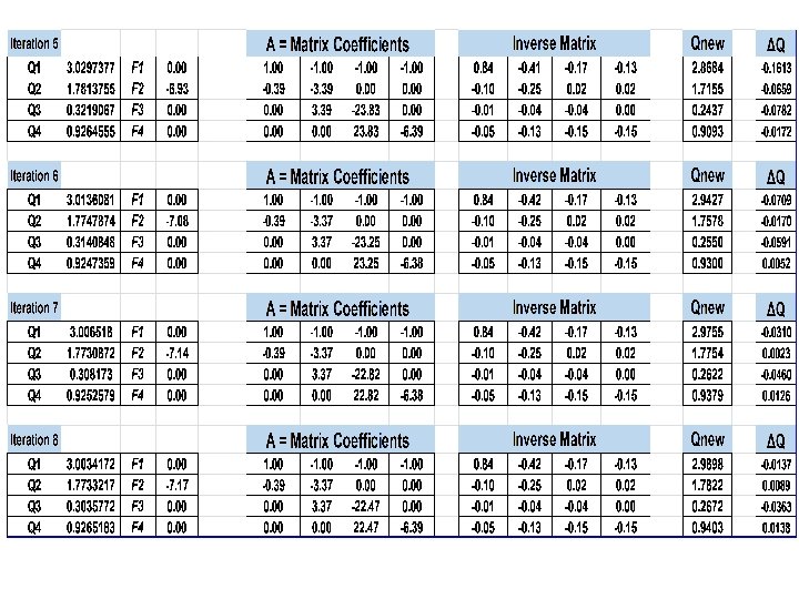
Example 8: Determine the flow distribution of water in the system shown in Fig. Assume constant friction factors, with f 0. 02. The head-discharge relation for the pump is HP = 60 10 Q 2. Solution [2] [1] [3]

All details of the solution are explained in the following table

Example 9: Find the water flow distribution in the parallel system shown in figure. The pump Power is 799. 68 Kw. Solution [I] [III] Assuming that , Q 1 = 2 , Q 2 = 1. 2, Q 3 = 0. 3 , Q 4 = 0. 5 Pipe L (m) D (mm) f ∑K 1 100 1200 0. 015 2 2 1000 0. 020 3 3 1500 0. 018 2 4 800 750 0. 021 4

All details of the solution are explained in the following table