Evolutionary Computation Genetic Algorithms Sources Material in this

Evolutionary Computation Genetic Algorithms

Sources • Material in this lecture comes from, “Handbook of Natural Computing, ” Editors Grzegorz Rosenberg, Thomas Back and Joost N. Kok, Springer 2014.

In set S In set X Coding function c: X S Decoding function is the inverse of c

• GAs manipulate coded versions of the problem parameters instead of the parameters themselves, i. e. , the search space is S instead of X • Conventional methods search from a single point while GAs operate on a whole population (reduces the risk of becoming trapped in a local extreme) • No use of auxiliary information about the objective function such as derivatives. GAs do need a meaningful decoding function • GAs use probabilistic transition operators while conventional methods for continuous optimization apply deterministic transition operators

312=52*6 evaluations of the fitness function

Conventional method likely gets stuck in a local maxima

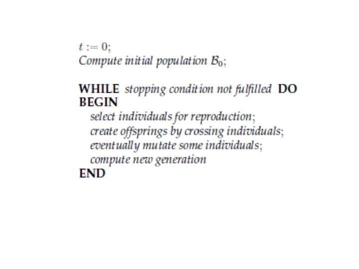
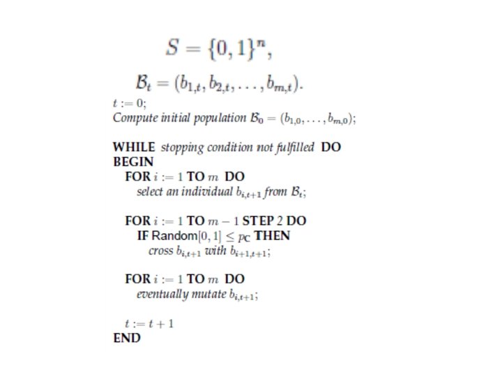
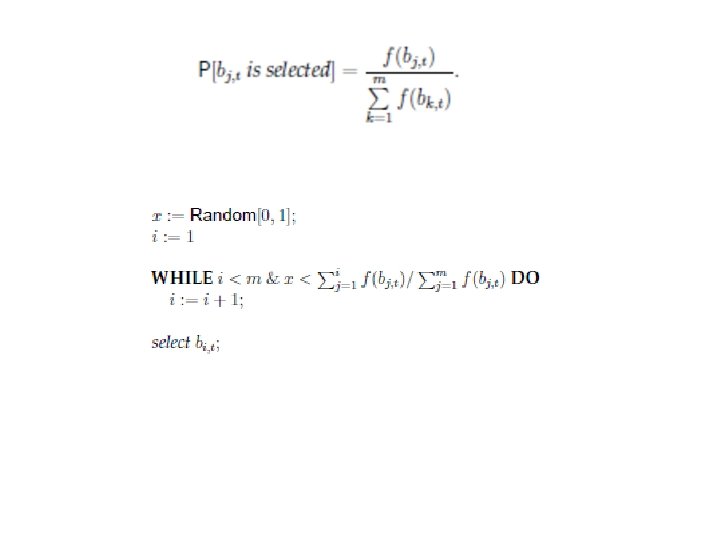
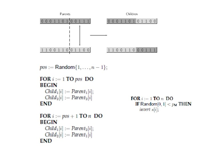
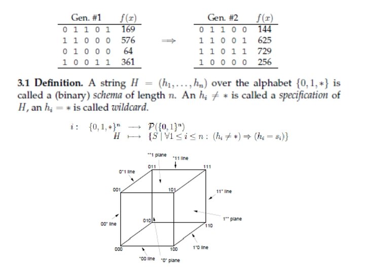
Roulette wheel selection One-point crossing over Bitwise mutation

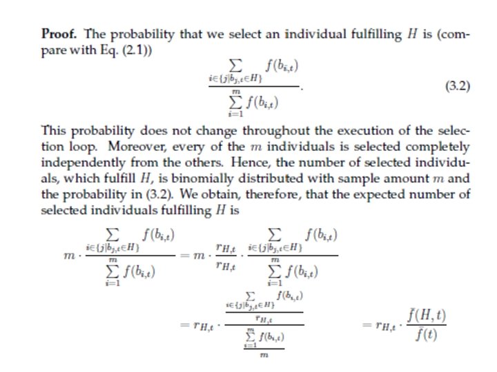
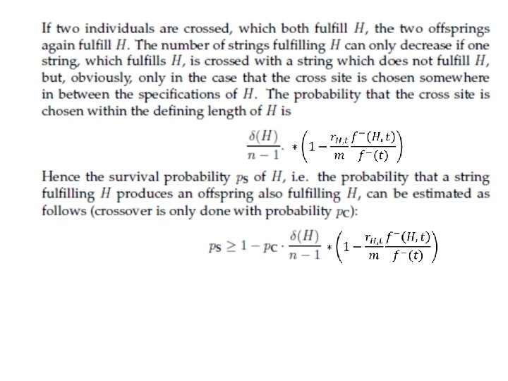
Schemata with above-average fitness and short defining length tend to produce more offspring than others: Called building blocks. The number of strings belonging to building blocks grows exponentially.

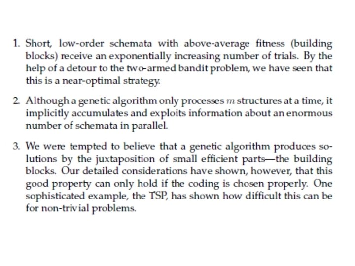
2 -armed bandit problem: left arm produces an outcome with mean mu_1 and variance sigma_1^2, right arm produces …. The optimal strategy is to allocate slightly more than an exponentially increasing number of trials to the observed best arm Consider the two schemata of order one which have their specification in the same position. The Schema theorem states that the GA implicitly decides between these two schemata based on incomplete data (observed average fitness values). GA solves a lot of 2 -armed bandit problems in parallel Schemata of higher order GA is solving an enormous number of k-armed bandit problems in parallel. Also here the observed better alternatives should receive an exponentially increasing number of trials and this us exactly what a GA does!

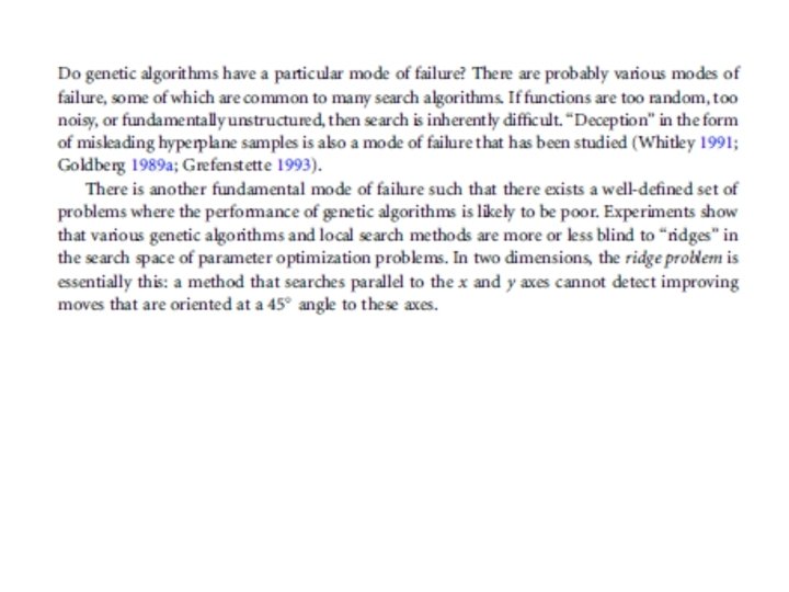
Criticism: • Schema theorem is an inequality • It only applies to one generation into the future: how do hyperplanes get sampled in the future? • 11*** and *00** have an inconsistency in the 2 nd bit: over multiple iterations both cannot receive increasing trials. The Schema theorem does not predict how such inconstistencies are sorted out. • Problems with a great deal of consistency (i. e. , the most fit schemata tend to agree) GA effective • GAs often use very small populations only smaller order schemata are sampled in reality (search relies more on hill climbing, which can be very effective) • Schema information up to any fixed order can be computed in polynomial time for some NP complete problem