Evolution of Reproductive Tactics semelparous versus iteroparous Reproductive

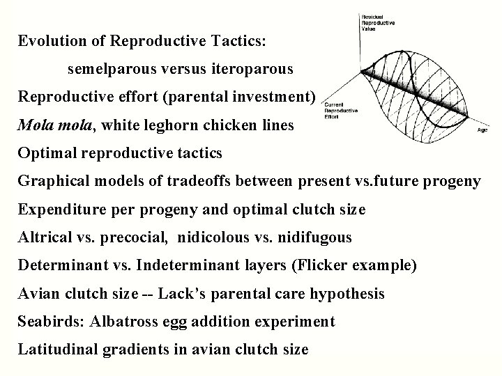
Evolution of Reproductive Tactics: semelparous versus iteroparous Reproductive effort (parental investment) Mola mola, white leghorn chicken lines Optimal reproductive tactics Graphical models of tradeoffs between present vs. future progeny Expenditure per progeny and optimal clutch size Altrical vs. precocial, nidicolous vs. nidifugous Determinant vs. Indeterminant layers (Flicker example) Avian clutch size -- Lack’s parental care hypothesis Seabirds: Albatross egg addition experiment Latitudinal gradients in avian clutch size

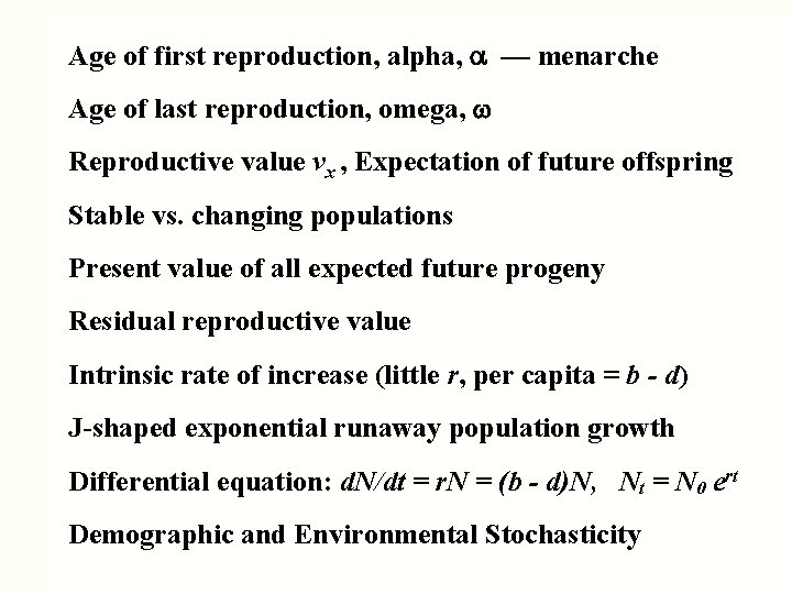
Age of first reproduction, alpha, — menarche Age of last reproduction, omega, Reproductive value vx , Expectation of future offspring Stable vs. changing populations Present value of all expected future progeny Residual reproductive value Intrinsic rate of increase (little r, per capita = b - d) J-shaped exponential runaway population growth Differential equation: d. N/dt = r. N = (b - d)N, Nt = N 0 ert Demographic and Environmental Stochasticity

Evolution of Reproductive Tactics Semelparous versus Interoparous Big Bang versus Repeated Reproduction Reproductive Effort (parental investment) Age of First Reproduction, alpha, a Age of Last Reproduction, omega,

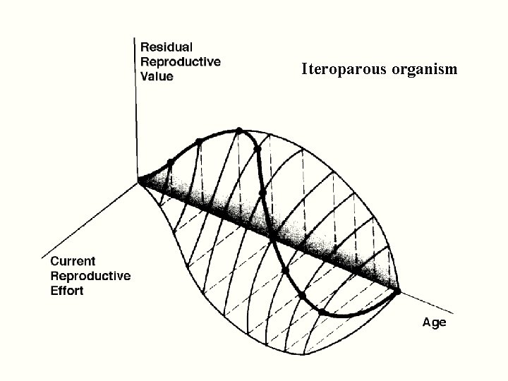
Iteroparous organism

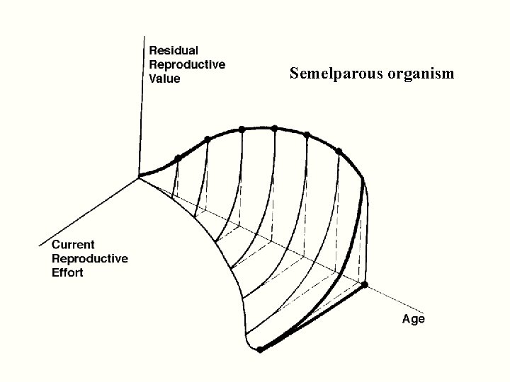
Semelparous organism

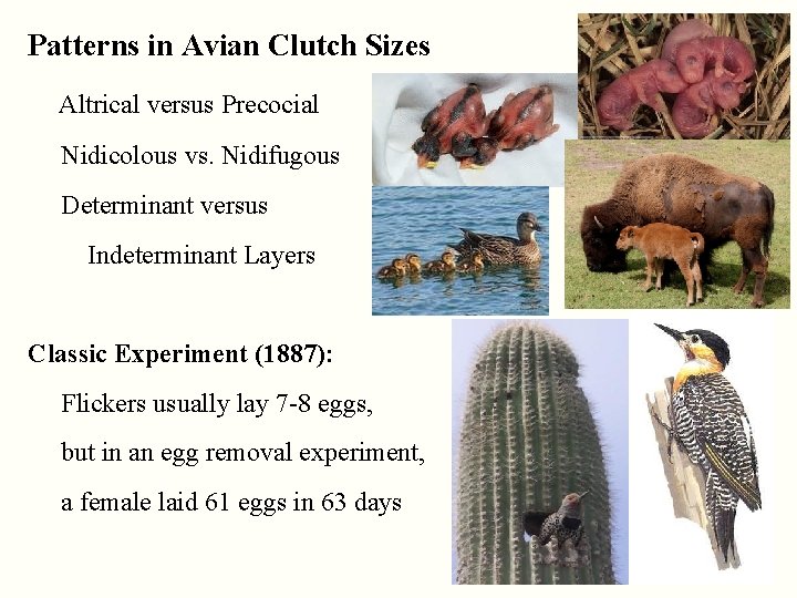
Patterns in Avian Clutch Sizes Altrical versus Precocial Nidicolous vs. Nidifugous Determinant versus Indeterminant Layers Classic Experiment (1887): Flickers usually lay 7 -8 eggs, but in an egg removal experiment, a female laid 61 eggs in 63 days

Great Tit Parus major David Lack

European Starling, Sturnus vulgaris David Lack

Chimney Swift, Apus apus David Lack

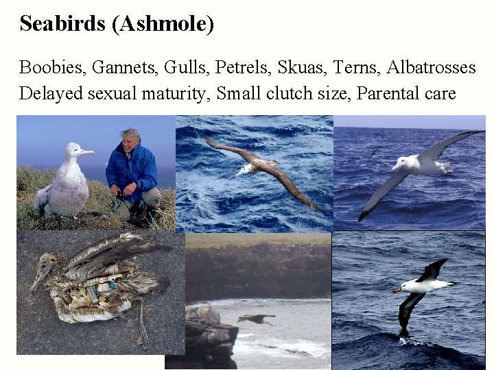
Seabirds (Ashmole) Boobies, Gannets, Gulls, Petrels, Skuas, Terns, Albatrosses Delayed sexual maturity, Small clutch size, Parental care

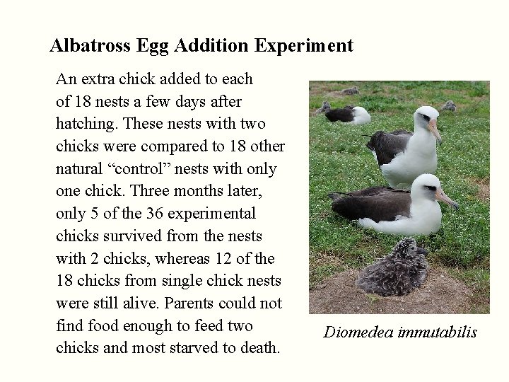
Albatross Egg Addition Experiment An extra chick added to each of 18 nests a few days after hatching. These nests with two chicks were compared to 18 other natural “control” nests with only one chick. Three months later, only 5 of the 36 experimental chicks survived from the nests with 2 chicks, whereas 12 of the 18 chicks from single chick nests were still alive. Parents could not find food enough to feed two chicks and most starved to death. Diomedea immutabilis

Latitudinal Gradients in Avian Clutch Size

Latitudinal Gradients in Avian Clutch Size Daylength Hypothesis Prey Diversity Hypothesis Spring Bloom or Competition Hypothesis

Latitudinal Gradients in Avian Clutch Size • Daylength Hypothesis • Prey Diversity Hypothesis (search images) • Spring Bloom or Competition Hypothesis • Nest Predation Hypothesis (Skutch) • Hazards of Migration Hypothesis

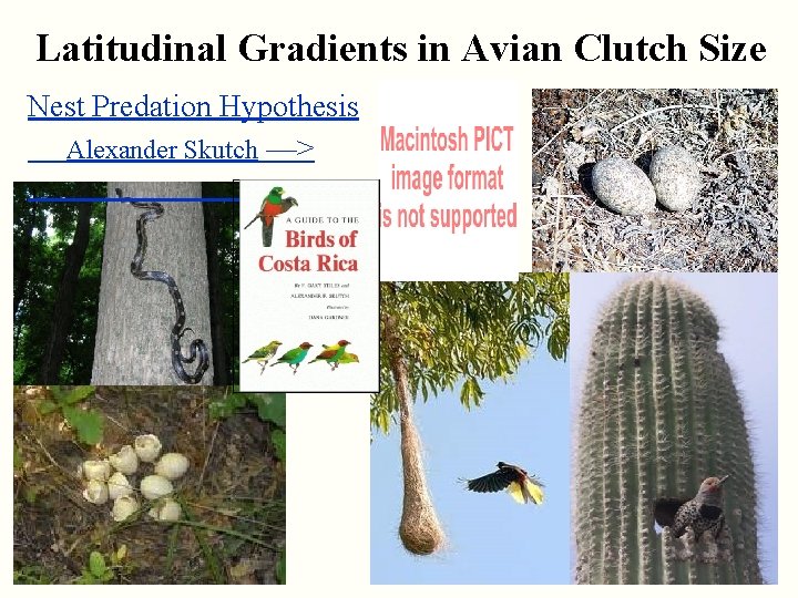
Latitudinal Gradients in Avian Clutch Size Nest Predation Hypothesis Alexander Skutch ––>

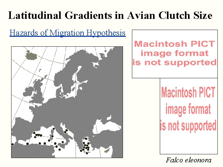
Latitudinal Gradients in Avian Clutch Size Hazards of Migration Hypothesis Falco eleonora

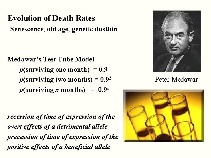
Evolution of Death Rates Senescence, old age, genetic dustbin Medawar’s Test Tube Model p(surviving one month) = 0. 9 p(surviving two months) = 0. 92 p(surviving x months) = 0. 9 x recession of time of expression of the overt effects of a detrimental allele precession of time of expression of the positive effects of a beneficial allele Peter Medawar

Age Distribution of Medawar’s test tubes Peter Medawar

Percentages of people with lactose intolerance

What starts off slow, finishes in a flash. . .

What starts off slow, finishes in a flash. . .

S - shaped sigmoidal population growth

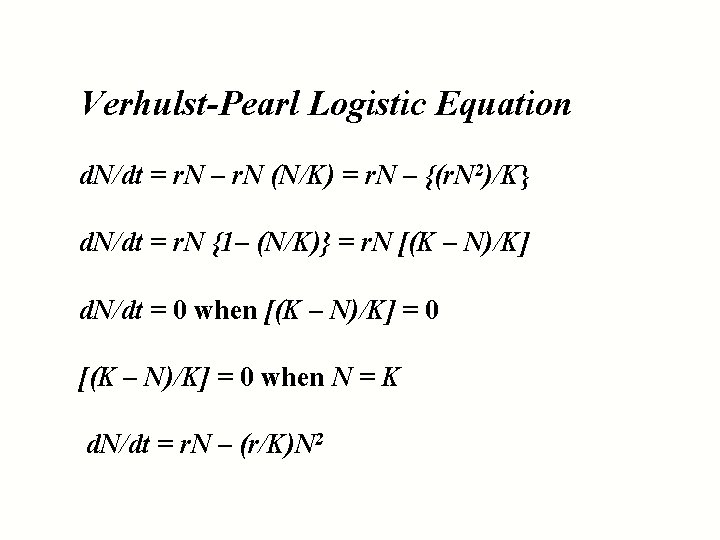
Verhulst-Pearl Logistic Equation d. N/dt = r. N – r. N (N/K) = r. N – {(r. N 2)/K} d. N/dt = r. N {1– (N/K)} = r. N [(K – N)/K] d. N/dt = 0 when [(K – N)/K] = 0 when N = K d. N/dt = r. N – (r/K)N 2

Inhibitory effect of each individual On its own population growth is 1/K

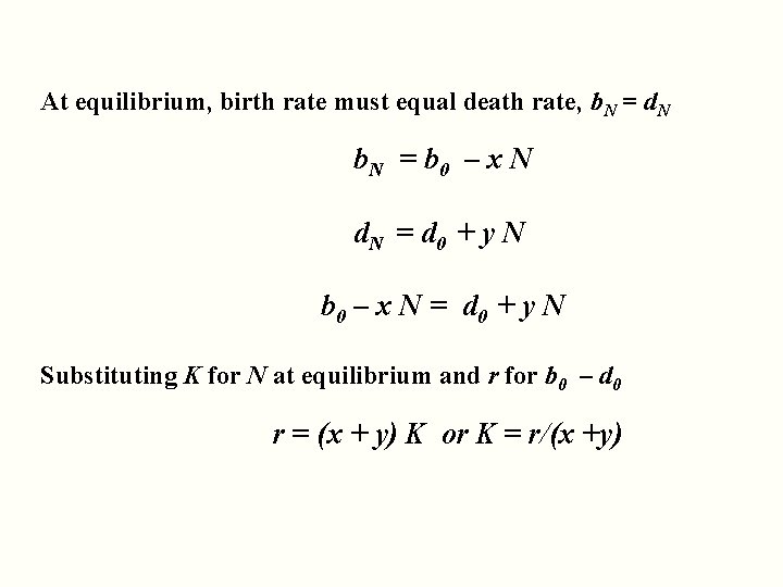
At equilibrium, birth rate must equal death rate, b. N = d. N b. N = b 0 – x N d. N = d 0 + y N b 0 – x N = d 0 + y N Substituting K for N at equilibrium and r for b 0 – d 0 r = (x + y) K or K = r/(x +y)

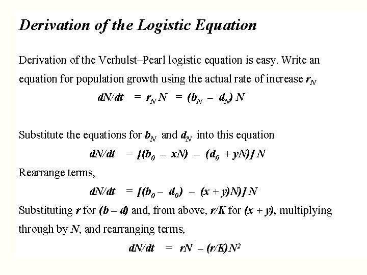
Derivation of the Logistic Equation Derivation of the Verhulst–Pearl logistic equation is easy. Write an equation for population growth using the actual rate of increase r. N d. N/dt = r. N N = (b. N – d. N) N Substitute the equations for b. N and d. N into this equation d. N/dt = [(b 0 – x. N) – (d 0 + y. N)] N Rearrange terms, d. N/dt = [(b 0 – d 0 ) – (x + y)N)] N Substituting r for (b – d) and, from above, r/K for (x + y), multiplying through by N, and rearranging terms, d. N/dt = r. N – (r/K)N 2