EViews Training Basic Estimation Time Series Models Note

EViews Training Basic Estimation: Time Series Models Note: Data and workfiles for this tutorial are provided in: ü Data: Data. xls ü Results: Results. wf 1 ü Practice Workfile: Data. wf 1

Data and Workfile Documentation • Data. wf 1 and Data. xls have monthly data from January 1960 -December 2011. ü M 1 – money supply, billions of USD (source: Board of Governors of the Federal Reserve) ü IP –industrial production, index levels (source: Board of Governors of the Federal Reserve) ü Tbill – 3 -month US Treasury rate (source: Board of Governors of the Federal Reserve) ü CPI – Consumer Price Index, level (source: Bureau of Labor Statistics) 2

Time Series Estimation • EViews has a built-in powerful toolkit that allows you to estimate time series models ranging from the simplest to the most complex types. • This tutorial demonstrates how to perform basic single equation time series regression techniques using EViews. • The main topics include: ü Specifying and Estimating Time Series Regressions ü Static and dynamic models ü Date functions ü Trends and seasonality ü Serial Correlation ü Testing for Serial Correlation ü Correcting for Serial Correlation: ARMA models ü Heteroskedasticity and Autocorrelation ü Testing for Heteroskedasticity and ARCH terms ü HAC Standard Errors ü Weighted Least Squares 3

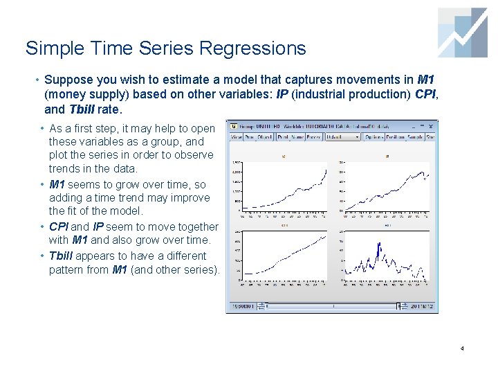
Simple Time Series Regressions • Suppose you wish to estimate a model that captures movements in M 1 (money supply) based on other variables: IP (industrial production) CPI, and Tbill rate. • As a first step, it may help to open these variables as a group, and plot the series in order to observe trends in the data. • M 1 seems to grow over time, so adding a time trend may improve the fit of the model. • CPI and IP seem to move together with M 1 and also grow over time. • Tbill appears to have a different pattern from M 1 (and other series). 4

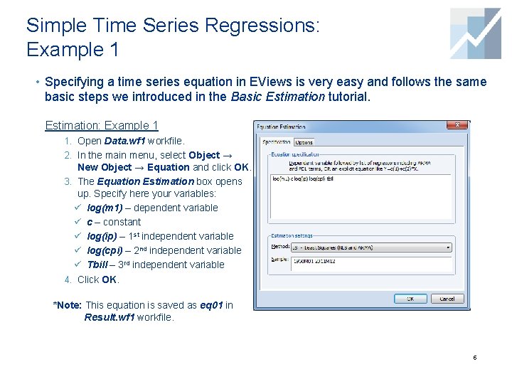
Simple Time Series Regressions: Example 1 • Specifying a time series equation in EViews is very easy and follows the same basic steps we introduced in the Basic Estimation tutorial. Estimation: Example 1 1. Open Data. wf 1 workfile. 2. In the main menu, select Object → New Object → Equation and click OK. 3. The Equation Estimation box opens up. Specify here your variables: ü log(m 1) – dependent variable ü c – constant ü log(ip) – 1 st independent variable ü log(cpi) – 2 nd independent variable ü Tbill – 3 rd independent variable 4. Click OK. *Note: This equation is saved as eq 01 in Result. wf 1 workfile. 5

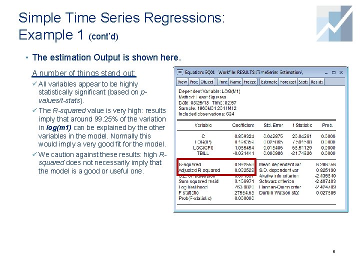
Simple Time Series Regressions: Example 1 (cont’d) • The estimation Output is shown here. A number of things stand out: ü All variables appear to be highly statistically significant (based on pvalues/t-stats). ü The R-squared value is very high: results imply that around 99. 25% of the variation in log(m 1) can be explained by the other variables in the model. Normally this would imply a very good fit for the model. ü We caution against these results: high Rsquared does not necessarily imply that the model is a good or useful one. 6

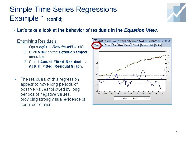
Simple Time Series Regressions: Example 1 (cont’d) • Let’s take a look at the behavior of residuals in the Equation View. Examining Residuals: 1. Open eq 01 in Results. wf 1 workfile. 2. Click View on the Equation Object menu bar. 3. Select Actual, Fitted, Residual → Actual, Fitted, Residual Graph. • The residuals of this regression appear to have long periods of positive values followed by long periods of negative values, providing strong visual evidence of serial correlation. 7

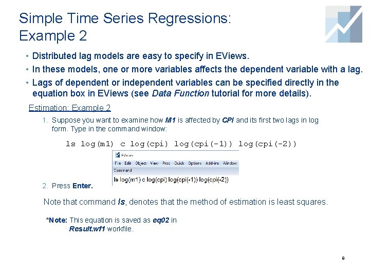
Simple Time Series Regressions: Example 2 • Distributed lag models are easy to specify in EViews. • In these models, one or more variables affects the dependent variable with a lag. • Lags of dependent or independent variables can be specified directly in the equation box in EViews (see Data Function tutorial for more details). Estimation: Example 2 1. Suppose you want to examine how M 1 is affected by CPI and its first two lags in log form. Type in the command window: ls log(m 1) c log(cpi) log(cpi(-1)) log(cpi(-2)) 2. Press Enter. Note that command ls, denotes that the method of estimation is least squares. *Note: This equation is saved as eq 02 in Result. wf 1 workfile. 8

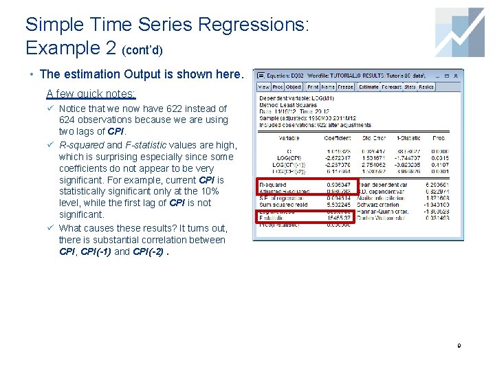
Simple Time Series Regressions: Example 2 (cont’d) • The estimation Output is shown here. A few quick notes: ü Notice that we now have 622 instead of 624 observations because we are using two lags of CPI. ü R-squared and F-statistic values are high, which is surprising especially since some coefficients do not appear to be very significant. For example, current CPI is statistically significant only at the 10% level, while the first lag of CPI is not significant. ü What causes these results? It turns out, there is substantial correlation between CPI, CPI(-1) and CPI(-2). 9

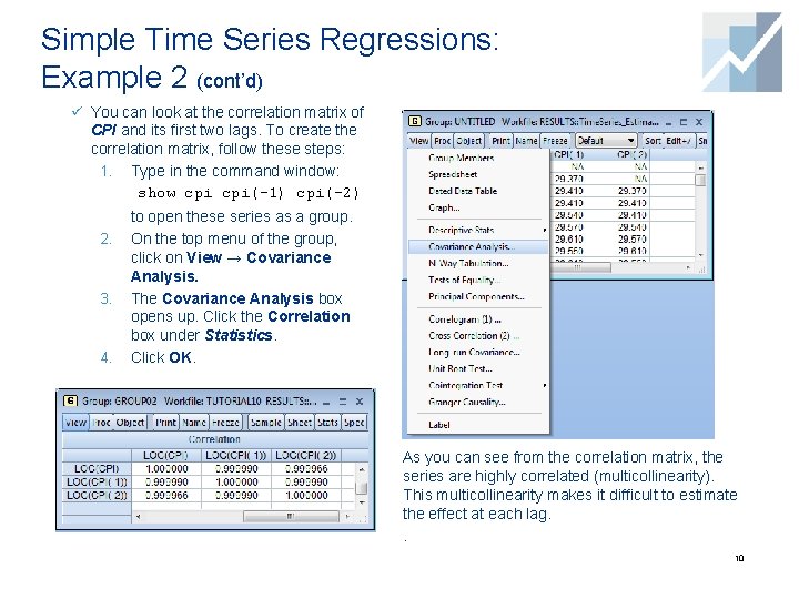
Simple Time Series Regressions: Example 2 (cont’d) ü You can look at the correlation matrix of CPI and its first two lags. To create the correlation matrix, follow these steps: 1. Type in the command window: show cpi(-1) cpi(-2) 2. 3. 4. to open these series as a group. On the top menu of the group, click on View → Covariance Analysis. The Covariance Analysis box opens up. Click the Correlation box under Statistics. Click OK. As you can see from the correlation matrix, the series are highly correlated (multicollinearity). This multicollinearity makes it difficult to estimate the effect at each lag. . 10

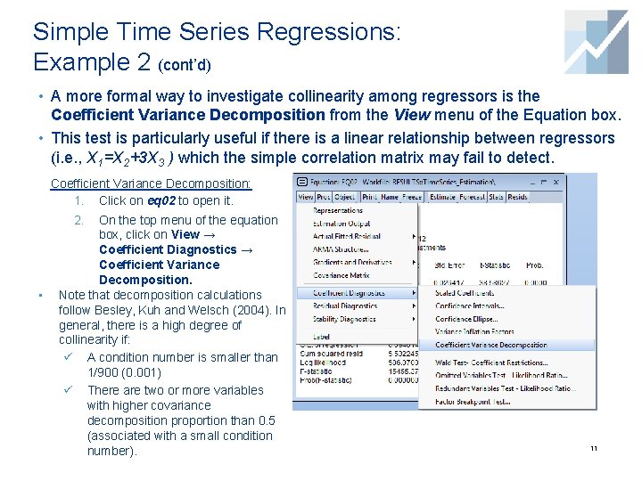
Simple Time Series Regressions: Example 2 (cont’d) • A more formal way to investigate collinearity among regressors is the Coefficient Variance Decomposition from the View menu of the Equation box. • This test is particularly useful if there is a linear relationship between regressors (i. e. , X 1=X 2+3 X 3 ) which the simple correlation matrix may fail to detect. Coefficient Variance Decomposition: 1. Click on eq 02 to open it. On the top menu of the equation box, click on View → Coefficient Diagnostics → Coefficient Variance Decomposition. Note that decomposition calculations follow Besley, Kuh and Welsch (2004). In general, there is a high degree of collinearity if: ü A condition number is smaller than 1/900 (0. 001) ü There are two or more variables with higher covariance decomposition proportion than 0. 5 (associated with a small condition number). 2. • 11

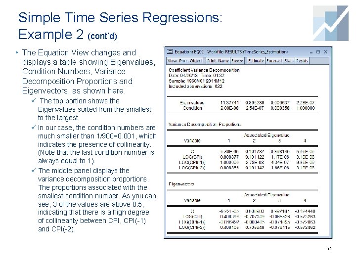
Simple Time Series Regressions: Example 2 (cont’d) • The Equation View changes and displays a table showing Eigenvalues, Condition Numbers, Variance Decomposition Proportions and Eigenvectors, as shown here. ü The top portion shows the Eigenvalues sorted from the smallest to the largest. ü In our case, the condition numbers are much smaller than 1/900=0. 001, which indicates the presence of collinearity. (Note that the last condition number is always equal to 1). ü The middle panel displays the variance decomposition proportions. The proportions associated with the smallest condition number. As you can see, 3 of the values are above 0. 5, indicating that there is a high degree of collinearity between CPI, CPI(-1) and CPI(-2). 12

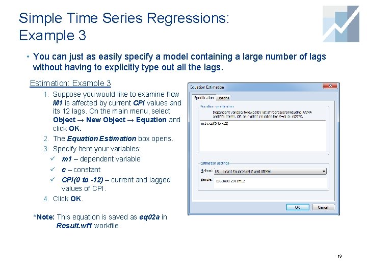
Simple Time Series Regressions: Example 3 • You can just as easily specify a model containing a large number of lags without having to explicitly type out all the lags. Estimation: Example 3 1. Suppose you would like to examine how M 1 is affected by current CPI values and its 12 lags. On the main menu, select Object → New Object → Equation and click OK. 2. The Equation Estimation box opens. 3. Specify here your variables: ü m 1 – dependent variable ü c – constant ü CPI(0 to -12) – current and lagged values of CPI. 4. Click OK. *Note: This equation is saved as eq 02 a in Result. wf 1 workfile. 13

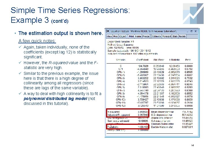
Simple Time Series Regressions: Example 3 (cont’d) • The estimation output is shown here. A few quick notes: ü Again, taken individually, none of the coefficients (except lag 12) is statistically significant. ü However, the R-squared value and the Fstatistic are very high. ü Similar to the previous example, the issue here is that there is a high degree of collinearity among all regressors (since these are lags of the same variable). ü A way to deal with high collinearity is to fit a polynomial distributed lag model (not discussed in this tutorial). 14

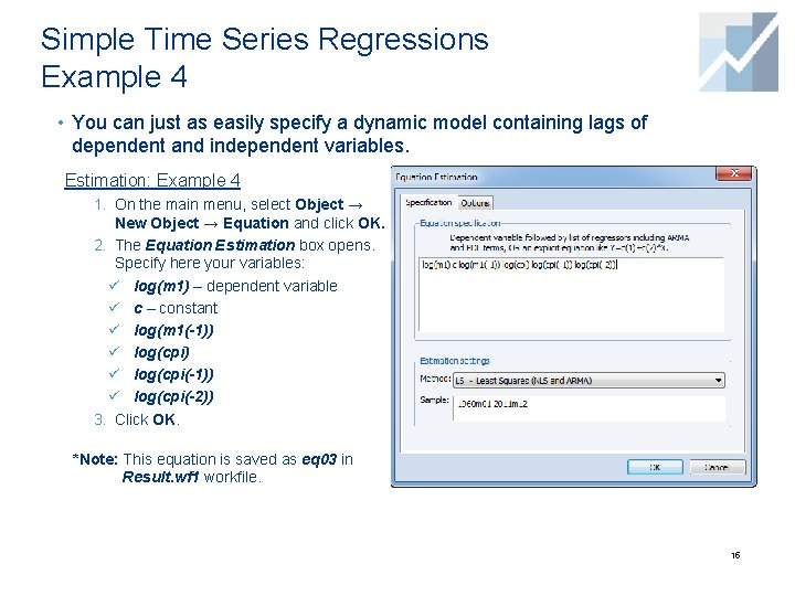
Simple Time Series Regressions Example 4 • You can just as easily specify a dynamic model containing lags of dependent and independent variables. Estimation: Example 4 1. On the main menu, select Object → New Object → Equation and click OK. 2. The Equation Estimation box opens. Specify here your variables: ü log(m 1) – dependent variable ü c – constant ü log(m 1(-1)) ü log(cpi(-1)) ü log(cpi(-2)) 3. Click OK. *Note: This equation is saved as eq 03 in Result. wf 1 workfile. 15

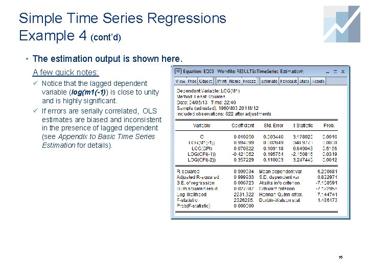
Simple Time Series Regressions Example 4 (cont’d) • The estimation output is shown here. A few quick notes: ü Notice that the lagged dependent variable (log(m 1(-1)) is close to unity and is highly significant. ü If errors are serially correlated, OLS estimates are biased and inconsistent in the presence of lagged dependent (see Appendix to Basic Time Series Estimation for details). 16

Time Series Models and Date Functions

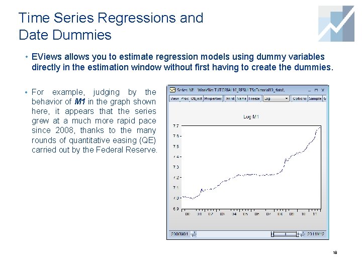
Time Series Regressions and Date Dummies • EViews allows you to estimate regression models using dummy variables directly in the estimation window without first having to create the dummies. • For example, judging by the behavior of M 1 in the graph shown here, it appears that the series grew at a much more rapid pace since 2008, thanks to the many rounds of quantitative easing (QE) carried out by the Federal Reserve. 18

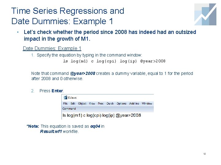
Time Series Regressions and Date Dummies: Example 1 • Let’s check whether the period since 2008 has indeed had an outsized impact in the growth of M 1. Date Dummies: Example 1 1. Specify the equation by typing in the command window: ls log(m 1) c log(cpi) log(ip) @year>2008 Note that command @year>2008 creates a dummy variable, equal to 1 for the period after 2008 and 0 otherwise. 2. Press Enter. *Note: This equation is saved as eq 04 in Result. wf 1 workfile. 19

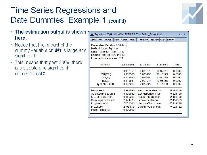
Time Series Regressions and Date Dummies: Example 1 (cont’d) • The estimation output is shown here. • Notice that the impact of the dummy variable on M 1 is large and significant. • This means that post-2008, there is a sizable and significant increase in M 1. 20

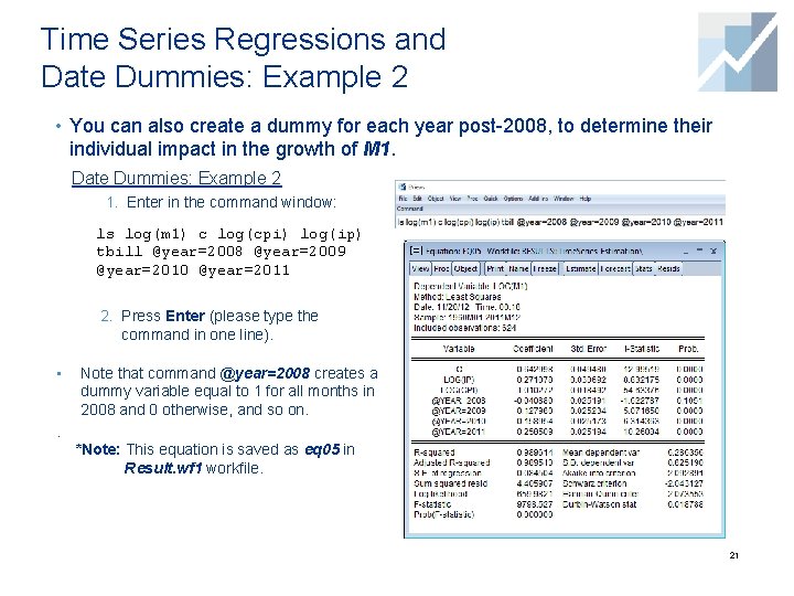
Time Series Regressions and Date Dummies: Example 2 • You can also create a dummy for each year post-2008, to determine their individual impact in the growth of M 1. Date Dummies: Example 2 1. Enter in the command window: ls log(m 1) c log(cpi) log(ip) tbill @year=2008 @year=2009 @year=2010 @year=2011 2. Press Enter (please type the command in one line). • . Note that command @year=2008 creates a dummy variable equal to 1 for all months in 2008 and 0 otherwise, and so on. *Note: This equation is saved as eq 05 in Result. wf 1 workfile. 21

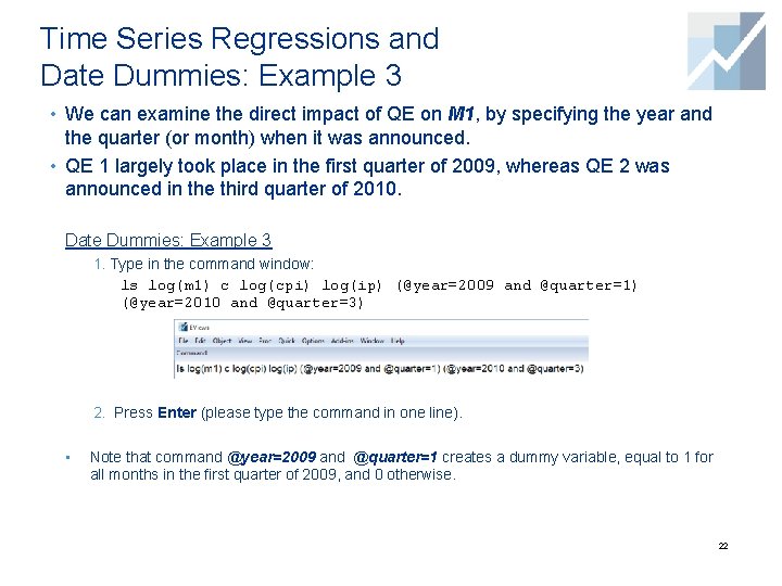
Time Series Regressions and Date Dummies: Example 3 • We can examine the direct impact of QE on M 1, by specifying the year and the quarter (or month) when it was announced. • QE 1 largely took place in the first quarter of 2009, whereas QE 2 was announced in the third quarter of 2010. Date Dummies: Example 3 1. Type in the command window: ls log(m 1) c log(cpi) log(ip) (@year=2009 and @quarter=1) (@year=2010 and @quarter=3) 2. Press Enter (please type the command in one line). • Note that command @year=2009 and @quarter=1 creates a dummy variable, equal to 1 for all months in the first quarter of 2009, and 0 otherwise. 22

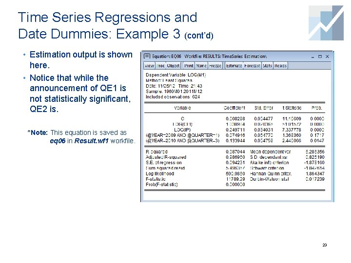
Time Series Regressions and Date Dummies: Example 3 (cont’d) • Estimation output is shown here. • Notice that while the announcement of QE 1 is not statistically significant, QE 2 is. *Note: This equation is saved as eq 06 in Result. wf 1 workfile. 23

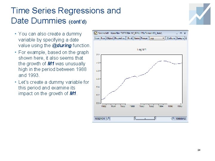
Time Series Regressions and Date Dummies (cont’d) • You can also create a dummy variable by specifying a date value using the @during function. • For example, based on the graph shown here, it also seems that the growth of M 1 was unusually high in the period between 1988 and 1993. • Let’s create a dummy variable for this period and examine its impact on the growth of M 1. 24

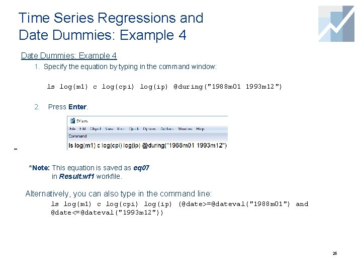
Time Series Regressions and Date Dummies: Example 4 1. Specify the equation by typing in the command window: ls log(m 1) c log(cpi) log(ip) @during("1988 m 01 1993 m 12") 2. Press Enter. *Note: This equation is saved as eq 07 in Result. wf 1 workfile. Alternatively, you can also type in the command line: ls log(m 1) c log(cpi) log(ip) (@date>=@dateval("1988 m 01") and @date<=@dateval("1993 m 12")) 25

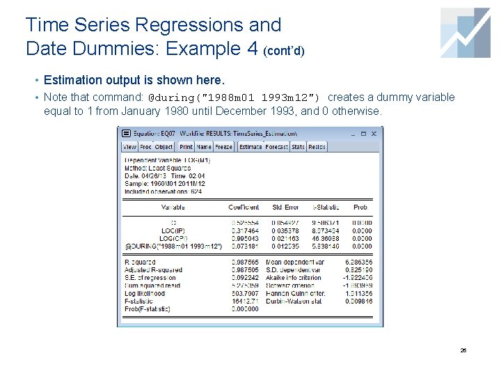
Time Series Regressions and Date Dummies: Example 4 (cont’d) • Estimation output is shown here. • Note that command: @during("1988 m 01 1993 m 12") creates a dummy variable equal to 1 from January 1980 until December 1993, and 0 otherwise. 26

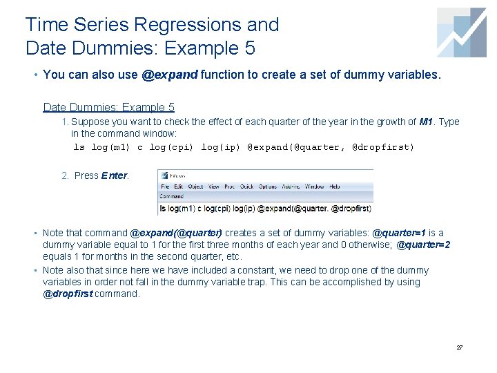
Time Series Regressions and Date Dummies: Example 5 • You can also use @expand function to create a set of dummy variables. Date Dummies: Example 5 1. Suppose you want to check the effect of each quarter of the year in the growth of M 1. Type in the command window: ls log(m 1) c log(cpi) log(ip) @expand(@quarter, @dropfirst) 2. Press Enter. • Note that command @expand(@quarter) creates a set of dummy variables: @quarter=1 is a dummy variable equal to 1 for the first three months of each year and 0 otherwise; @quarter=2 equals 1 for months in the second quarter, etc. • Note also that since here we have included a constant, we need to drop one of the dummy variables in order not fall in the dummy variable trap. This can be accomplished by using @dropfirst command. 27

Trends and Seasonality

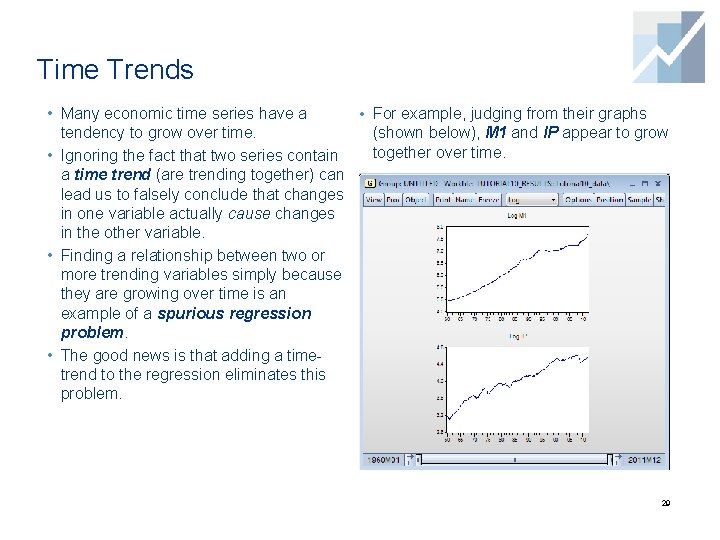
Time Trends • Many economic time series have a • For example, judging from their graphs tendency to grow over time. (shown below), M 1 and IP appear to grow together over time. • Ignoring the fact that two series contain a time trend (are trending together) can lead us to falsely conclude that changes in one variable actually cause changes in the other variable. • Finding a relationship between two or more trending variables simply because they are growing over time is an example of a spurious regression problem. • The good news is that adding a timetrend to the regression eliminates this problem. 29

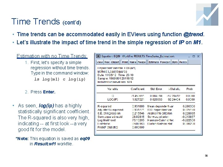
Time Trends (cont’d) • Time trends can be accommodated easily in EViews using function @trend. • Let’s illustrate the impact of time trend in the simple regression of IP on M 1. Estimation with no Time Trends: 1. First, let’s specify a simple regression without time trends. Type in the command window: ls log(m 1) c log(ip) 2. Press Enter. • As seen, log(ip) has a highly statistically significant coefficient. The R-squared is also very high, indicating -- at first look --a very good fit for the model. *Note: This equation is saved as eq 09 in Result. wf 1 workfile. 30

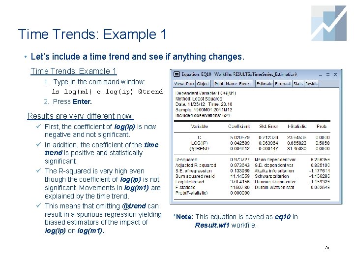
Time Trends: Example 1 • Let’s include a time trend and see if anything changes. Time Trends: Example 1 1. Type in the command window: ls log(m 1) c log(ip) @trend 2. Press Enter. Results are very different now: ü First, the coefficient of log(ip) is now negative and not significant. ü In addition, the coefficient of the time trend is positive and statistically significant. ü The R-squared is very high even though the coefficient of log(ip) is not significant. Movements in log(m 1) are explained by the time trend. ü This means that omitting @trend can result in a spurious regression yielding biased estimators of the impact of log(ip) on log(m 1). *Note: This equation is saved as eq 10 in Result. wf 1 workfile. 31

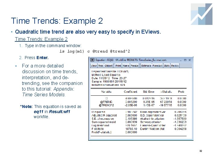
Time Trends: Example 2 • Quadratic time trend are also very easy to specify in EViews. Time Trends: Example 2 1. Type in the command window: ls log(m 1) c @trend^2 2. Press Enter. • For a more detailed discussion on time trends, interpretation, and detrending, see the companion to this tutorial: Appendix: Time Series Models. *Note: This equation is saved as eq 11 in Result. wf 1 workfile. 32

Seasonality • Sometimes time series exhibit seasonal patterns. For example, retails sales tend to be higher in the last quarter of the year because of the Holiday Shopping season. • Most macroeconomic series are already seasonally adjusted beforehand so there is no need to worry about seasonal issues. • If you suspect a series displays seasonal patterns, you can include a set of dummy variables to account for the seasonality in the dependent variable. • EViews has a built-in function that creates dummy variables corresponding to each month (or quarter, if the data is quarterly). 33

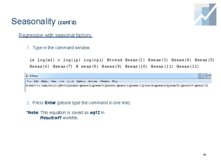
Seasonality (cont’d) Regression with seasonal factors: 1. Type in the command window: ls log(m 1) c log(ip) log(cpi) @trend @seas(2) @seas(3) @seas(4) @seas(5) @seas(6) @seas(7) @ seas(8) @seas(9) @seas(10) @seas(11) @seas(12) 2. Press Enter (please type the command in one line). *Note: This equation is saved as eq 12 in Result. wf 1 workfile. 34

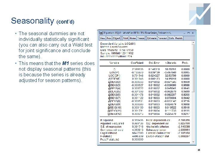
Seasonality (cont’d) • The seasonal dummies are not individually statistically significant (you can also carry out a Wald test for joint significance and conclude the same). • This means that the M 1 series does not display seasonal patterns (this is because the series is already adjusted for season patterns). 35

Testing for Serial Correlation

Serial Correlation • As we have seen in the previous examples, residuals from our time series regressions appear to be correlated with their own lagged values (they display serial correlation). • Serial correlation is a common occurrence in time series data because the data is ordered (over time); it is therefore not surprising that neighboring error terms turn out to be correlated. • Serial correlation violates the standard assumption of regression theory that error terms are uncorrelated. 37

Serial Correlation (cont’d) • If untreated, serial correlation leads to a number of issues: ü Reported standard errors and t-statistics are invalid (even asymptotically). ü Coefficients may be biased, though not necessarily inconsistent (if data is weakly dependent). ü In the presence of lagged dependent variables, OLS estimates are biased and inconsistent. • Fortunately, EViews provides tools for detecting serial correlation and correcting regressions to account for its presence. Note: in the following examples we will treat serial correlation as a statistical issue. However, serial correlation is sometimes a hint of model misspecification. Though we don’t investigate this here, misspecification is likely an issue in the following examples. 38

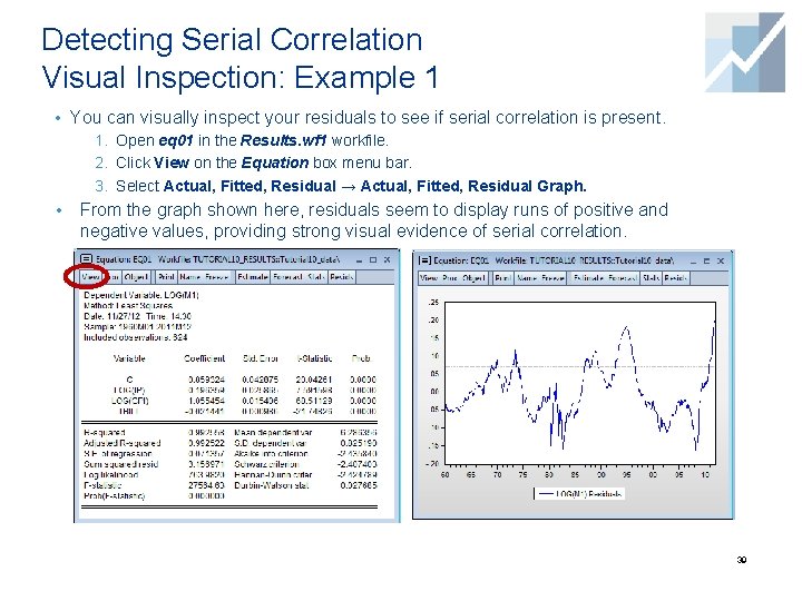
Detecting Serial Correlation Visual Inspection: Example 1 • You can visually inspect your residuals to see if serial correlation is present. 1. Open eq 01 in the Results. wf 1 workfile. 2. Click View on the Equation box menu bar. 3. Select Actual, Fitted, Residual → Actual, Fitted, Residual Graph. • From the graph shown here, residuals seem to display runs of positive and negative values, providing strong visual evidence of serial correlation. 39

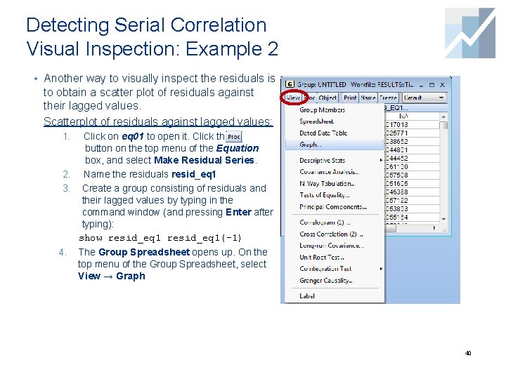
Detecting Serial Correlation Visual Inspection: Example 2 • Another way to visually inspect the residuals is to obtain a scatter plot of residuals against their lagged values. Scatterplot of residuals against lagged values: Click on eq 01 to open it. Click the button on the top menu of the Equation box, and select Make Residual Series. 2. Name the residuals resid_eq 1 3. Create a group consisting of residuals and their lagged values by typing in the command window (and pressing Enter after typing): show resid_eq 1(-1) 1. 4. The Group Spreadsheet opens up. On the top menu of the Group Spreadsheet, select View → Graph 40

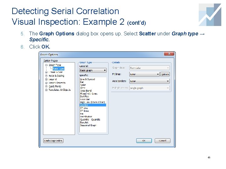
Detecting Serial Correlation Visual Inspection: Example 2 (cont’d) 5. The Graph Options dialog box opens up. Select Scatter under Graph type → Specific. 6. Click OK. 41

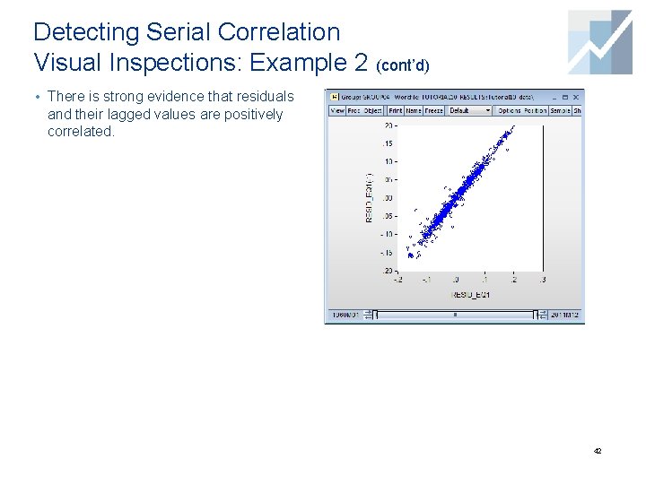
Detecting Serial Correlation Visual Inspections: Example 2 (cont’d) • There is strong evidence that residuals and their lagged values are positively correlated. 42

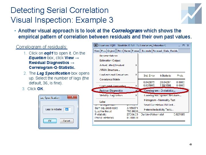
Detecting Serial Correlation Visual Inspection: Example 3 • Another visual approach is to look at the Correlogram which shows the empirical pattern of correlation between residuals and their own past values. Correlogram of residuals: 1. Click on eq 01 to open it. On the Equation box, click View → Residual Diagnostics → Correlogram-Q-Statistic. 2. The Lag Specification box opens up. Select the number of lags (the default, 36, is fine). 3. Click OK. 43

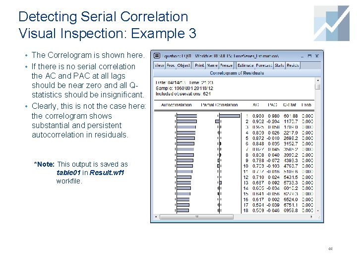
Detecting Serial Correlation Visual Inspection: Example 3 • The Correlogram is shown here. • If there is no serial correlation the AC and PAC at all lags should be near zero and all Qstatistics should be insignificant. • Clearly, this is not the case here: the correlogram shows substantial and persistent autocorrelation in residuals. *Note: This output is saved as table 01 in Result. wf 1 workfile. 44

Testing for Serial Correlation in EViews • Visual checks provide important information, but we may want to carry out formal tests for serial correlation. • EViews provides three test statistics: 1. Durbin-Watson 2. Breusch-Godfrey 3. Ljung-Box Q-Statistic (or the correlogram; explained above). 45

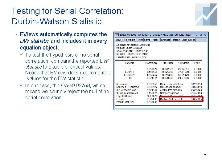
Testing for Serial Correlation: Durbin-Watson Statistic • EViews automatically computes the DW statistic and includes it in every equation object. ü To test the hypothesis of no serial correlation, compare the reported DW statistic to a table of critical values. Notice that EViews does not compute p -values for the DW statistic. ü In our case, the DW=0. 02768, which means we soundly reject the null of no serial correlation. 46

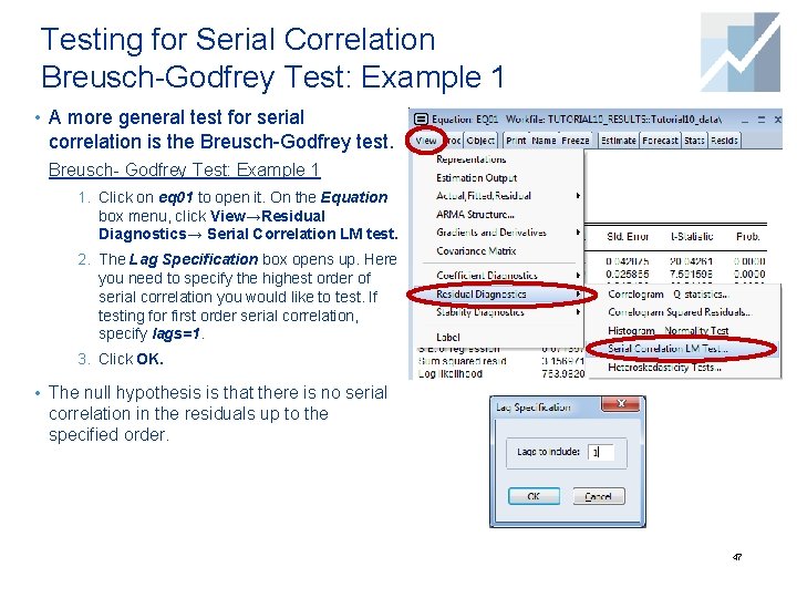
Testing for Serial Correlation Breusch-Godfrey Test: Example 1 • A more general test for serial correlation is the Breusch-Godfrey test. Breusch- Godfrey Test: Example 1 1. Click on eq 01 to open it. On the Equation box menu, click View→Residual Diagnostics→ Serial Correlation LM test. 2. The Lag Specification box opens up. Here you need to specify the highest order of serial correlation you would like to test. If testing for first order serial correlation, specify lags=1. 3. Click OK. • The null hypothesis is that there is no serial correlation in the residuals up to the specified order. 47

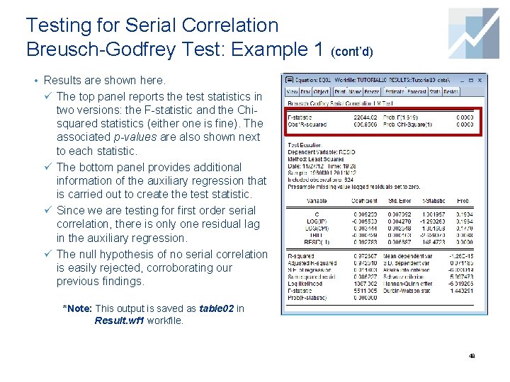
Testing for Serial Correlation Breusch-Godfrey Test: Example 1 (cont’d) • Results are shown here. ü The top panel reports the test statistics in two versions: the F-statistic and the Chisquared statistics (either one is fine). The associated p-values are also shown next to each statistic. ü The bottom panel provides additional information of the auxiliary regression that is carried out to create the test statistic. ü Since we are testing for first order serial correlation, there is only one residual lag in the auxiliary regression. ü The null hypothesis of no serial correlation is easily rejected, corroborating our previous findings. *Note: This output is saved as table 02 in Result. wf 1 workfile. 48

Correcting for Serial Correlation: ARMA Models

Correcting for Serial Correlation • If you detect serial correlation, something needs to be done. • Serial correlation in the error term may be evidence of a serious problem of model misspecification. • If your goal is to estimate a model with complete dynamics, you need to respecify the model. • If you do not wish to estimate a fully dynamic model, but would like to carry out statistical inference, then you need to account for serial correlation so that test statistics are valid. • EViews has built-in features to correct for either autoregressive (AR(p)) or moving average (MA(q)) errors, or both. 50

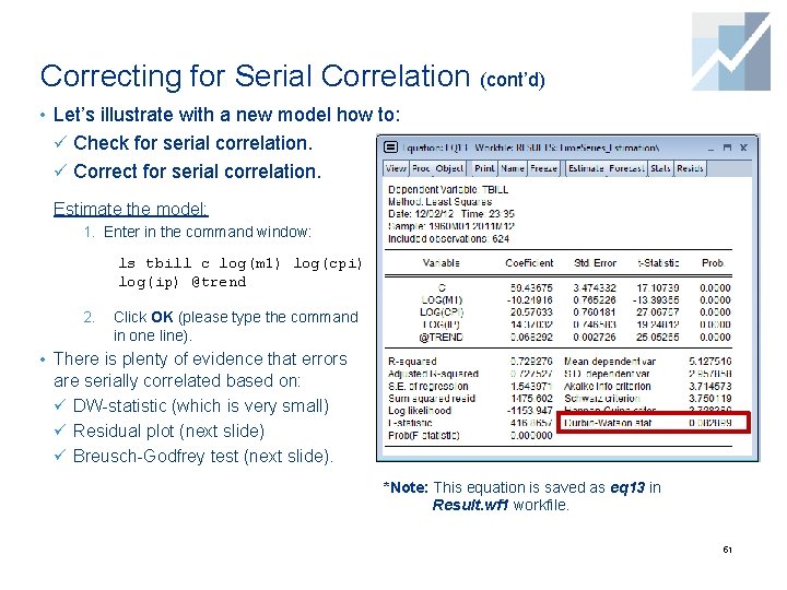
Correcting for Serial Correlation (cont’d) • Let’s illustrate with a new model how to: ü Check for serial correlation. ü Correct for serial correlation. Estimate the model: 1. Enter in the command window: ls tbill c log(m 1) log(cpi) log(ip) @trend 2. Click OK (please type the command in one line). • There is plenty of evidence that errors are serially correlated based on: ü DW-statistic (which is very small) ü Residual plot (next slide) ü Breusch-Godfrey test (next slide). *Note: This equation is saved as eq 13 in Result. wf 1 workfile. 51

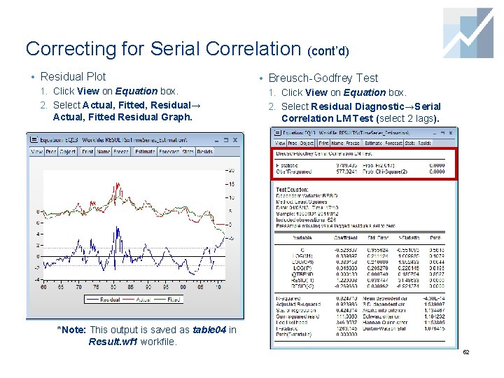
Correcting for Serial Correlation (cont’d) • Residual Plot • Breusch-Godfrey Test 1. Click View on Equation box. 2. Select Actual, Fitted, Residual→ 2. Select Residual Diagnostic→Serial Actual, Fitted Residual Graph. Correlation LM Test (select 2 lags). *Note: This output is saved as table 04 in Result. wf 1 workfile. 52

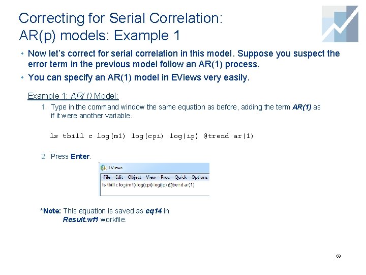
Correcting for Serial Correlation: AR(p) models: Example 1 • Now let’s correct for serial correlation in this model. Suppose you suspect the error term in the previous model follow an AR(1) process. • You can specify an AR(1) model in EViews very easily. Example 1: AR(1) Model: 1. Type in the command window the same equation as before, adding the term AR(1) as if it were another variable. ls tbill c log(m 1) log(cpi) log(ip) @trend ar(1) 2. Press Enter. *Note: This equation is saved as eq 14 in Result. wf 1 workfile. 53

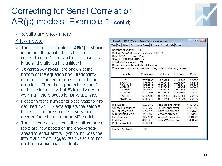
Correcting for Serial Correlation AR(p) models: Example 1 (cont’d) • Results are shown here. A few notes: ü The coefficient estimate for AR(1) is shown in the middle panel. This is the serial correlation coefficient and in our case it is large and statistically significant. ü “Inverted AR roots” are shown at the bottom of the equation box. Stationarity requires that inverted roots lie inside the unit circle. There is no particular issue if roots are imaginary, but EViews issues a warning if the process is non-stationary. ü Notice that the number of observations has declined by 1; EViews adjusts the sample to free up the pre-sample observation needed for estimation of an AR model. ü The summary statistics at the bottom of the table are now based on the one-periodahead forecast errors (which includes the information from lagged residuals) and not on the unconditional residuals. 54

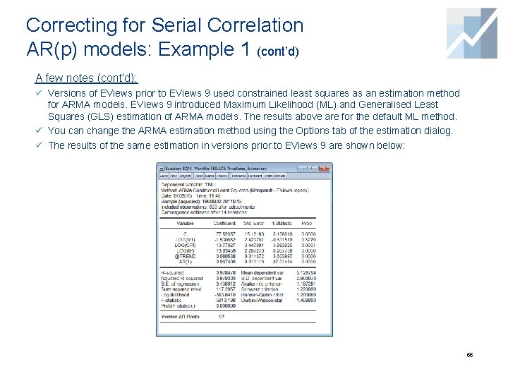
Correcting for Serial Correlation AR(p) models: Example 1 (cont’d) A few notes (cont'd): ü Versions of EViews prior to EViews 9 used constrained least squares as an estimation method for ARMA models. EViews 9 introduced Maximum Likelihood (ML) and Generalised Least Squares (GLS) estimation of ARMA models. The results above are for the default ML method. ü You can change the ARMA estimation method using the Options tab of the estimation dialog. ü The results of the same estimation in versions prior to EViews 9 are shown below: 55

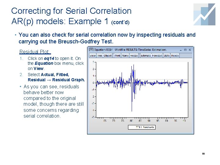
Correcting for Serial Correlation AR(p) models: Example 1 (cont’d) • You can also check for serial correlation now by inspecting residuals and carrying out the Breusch-Godfrey Test. Residual Plot: 1. 2. Click on eq 14 to open it. On the Equation box menu, click on View. Select Actual, Fitted, Residual → Residual Graph. • As you can see, residuals behave better now compared to the original model, though there are still some concerns regarding serial correlation. 56

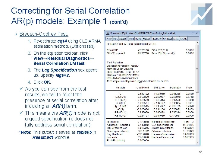
Correcting for Serial Correlation AR(p) models: Example 1 (cont’d) • Breusch-Godfrey Test: 1. Re-estimate eq 14 using CLS ARMA estimation method. (Options tab) 2. On the equation toolbar, click View→Residual Diagnostics→ Serial Correlation LM test. 3. The Lag Specification box opens up. Specify lags=2. 4. Click OK. ü As you can see from the test results, we fail to reject the presence of serial correlation after including an AR(1) term. ü This means the AR(1) model is not a good specification (it does not fully address serial correlation). *Note: This output is saved as table 05 in Result. wf 1 workfile. 57

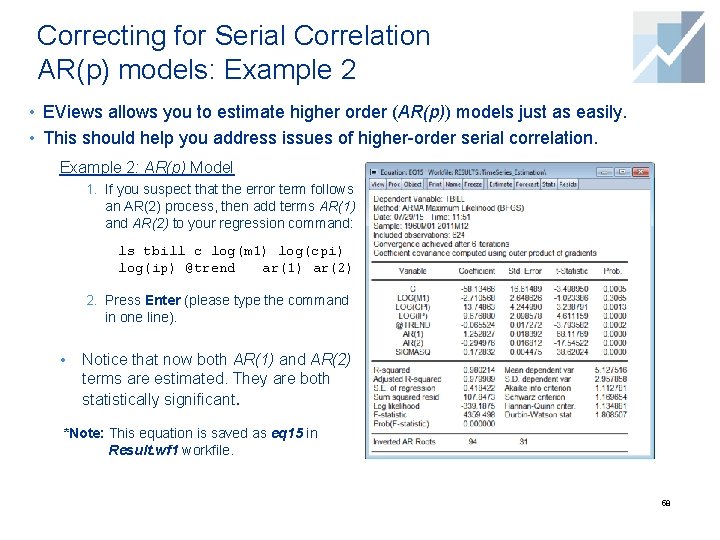
Correcting for Serial Correlation AR(p) models: Example 2 • EViews allows you to estimate higher order (AR(p)) models just as easily. • This should help you address issues of higher-order serial correlation. Example 2: AR(p) Model 1. If you suspect that the error term follows an AR(2) process, then add terms AR(1) and AR(2) to your regression command: ls tbill c log(m 1) log(cpi) log(ip) @trend ar(1) ar(2) 2. Press Enter (please type the command in one line). • Notice that now both AR(1) and AR(2) terms are estimated. They are both statistically significant. *Note: This equation is saved as eq 15 in Result. wf 1 workfile. 58

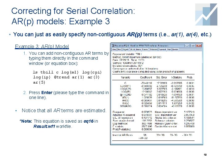
Correcting for Serial Correlation: AR(p) models: Example 3 • You can just as easily specify non-contiguous AR(p) terms (i. e. , ar(1), ar(4), etc. ) Example 3: AR(p) Model 1. You can add non-contiguous AR terms by typing them directly in the command window (or equation box): ls tbill c log(m 1) log(cpi) log(ip) @trend ar(1) ar(3) ar(5) 2. Press Enter (please type the command in one line). • Notice that all AR terms are estimated. *Note: This equation is saved as eq 16 in Result. wf 1 workfile. 59

Correcting for Serial Correlation: AR(p) models (cont’d) A couple of additional notes: ü As shown above, EViews allows you to include non-contiguous AR terms (ar(2) ar(4), etc. ) ü The downside to this is that if you are estimating a higher-order AR process, EViews requires you to include all lower-order terms. For example, to estimate an AR(3) model, you need to include: ar(1) ar(2) a(3) (or, in EViews 8, ar(1 to 3)). ü If you simply type ar(3) and omit other terms, this forces the estimate of ar(1) and ar(2) to zero. You may want this on rare occasions (for example, when dealing with seasonal components), but not on a routine basis. 60

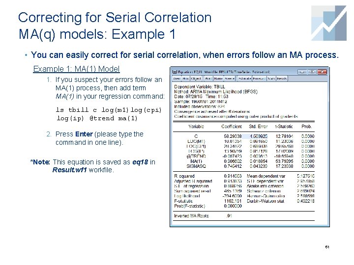
Correcting for Serial Correlation MA(q) models: Example 1 • You can easily correct for serial correlation, when errors follow an MA process. Example 1: MA(1) Model 1. If you suspect your errors follow an MA(1) process, then add term MA(1) in your regression command: ls tbill c log(m 1)log(cpi) log(ip) @trend ma(1) 2. Press Enter (please type the command in one line). *Note: This equation is saved as eq 18 in Result. wf 1 workfile. 61

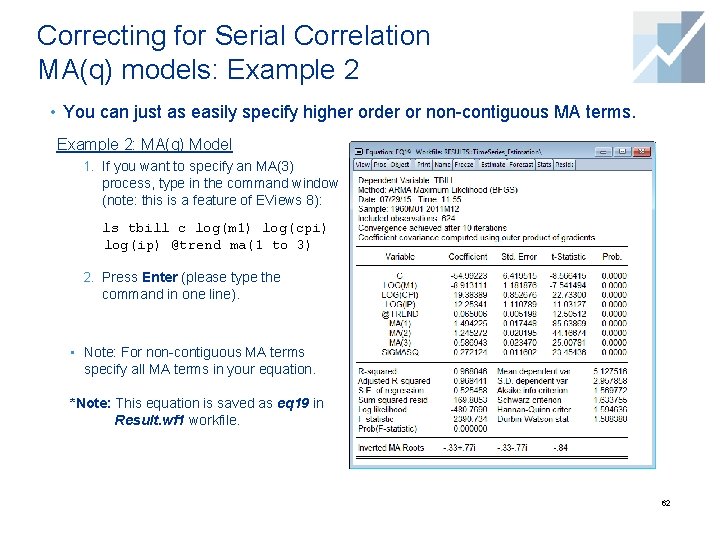
Correcting for Serial Correlation MA(q) models: Example 2 • You can just as easily specify higher order or non-contiguous MA terms. Example 2: MA(q) Model 1. If you want to specify an MA(3) process, type in the command window (note: this is a feature of EViews 8): ls tbill c log(m 1) log(cpi) log(ip) @trend ma(1 to 3) 2. Press Enter (please type the command in one line). • Note: For non-contiguous MA terms specify all MA terms in your equation. *Note: This equation is saved as eq 19 in Result. wf 1 workfile. 62

Correcting for Serial Correlation: MA(q) models (cont’d) Some additional notes: ü As it must be obvious by now, if your errors follow an MA(2) process, you need to include both ma(1) and ma(2) terms in the regression. ü Unlike nearly all other EViews estimation procedures, MA models require a continuous sample. If your sample includes a break or has missing data (NA values), EViews will give an error message. ü Notice that in general, MA models are notoriously difficult to estimate. In particular, higher order MA terms should be avoided unless absolutely required for your model. 63

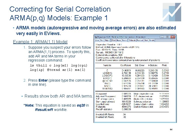
Correcting for Serial Correlation ARMA(p, q) Models: Example 1 • ARMA models (autoregressive and moving average errors) are also estimated very easily in EViews. Example 1: ARMA(1, 1) Model 1. Suppose you suspect your errors follow an ARMA(1, 1) process. To specify this, add AR and MA terms in your regression command: ls tbill c log(m 1) log(cpi) log(ip) @trend ar(1) ma(1) 2. Press Enter (please type the command in one line). • Results show both AR and MA terms. *Note: This equation is saved as eq 20 in Result. wf 1 workfile. 64

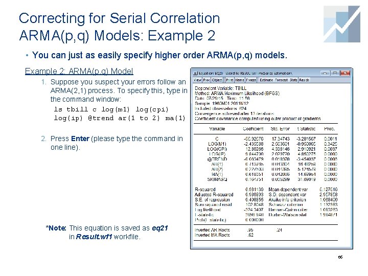
Correcting for Serial Correlation ARMA(p, q) Models: Example 2 • You can just as easily specify higher order ARMA(p, q) models. Example 2: ARMA(p, q) Model 1. Suppose you suspect your errors follow an ARMA(2, 1) process. To specify this, type in the command window: ls tbill c log(m 1) log(cpi) log(ip) @trend ar(1 to 2) ma(1) 2. Press Enter (please type the command in one line). *Note: This equation is saved as eq 21 in Result. wf 1 workfile. 65

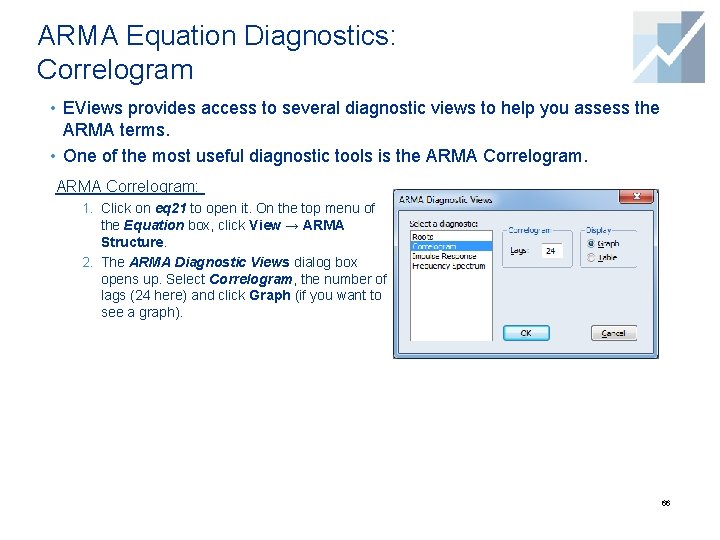
ARMA Equation Diagnostics: Correlogram • EViews provides access to several diagnostic views to help you assess the ARMA terms. • One of the most useful diagnostic tools is the ARMA Correlogram: 1. Click on eq 21 to open it. On the top menu of the Equation box, click View → ARMA Structure. 2. The ARMA Diagnostic Views dialog box opens up. Select Correlogram, the number of lags (24 here) and click Graph (if you want to see a graph). 66

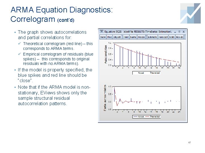
ARMA Equation Diagnostics: Correlogram (cont’d) • The graph shows autocorrelations and partial correlations for: ü Theoretical correlogram (red line) – this corresponds to ARMA terms. ü Empirical correlogram of residuals (blue spikes) -- this corresponds to original residuals with no ARMA terms). • If the model is properly specified, the blue spikes and red line should be “close”. • Note that if the ARMA model is nonstationary, EViews shows only the sample structural residual autocorrelation patterns. 67

Differencing and Serial Correlation • An alternative way to deal with serial correlation is to difference the data. • In fact, differencing the data (e. g. , taking first-order differences) addresses a number of issues that arise in time series data: ü It eliminates most (perhaps not all) serial correlation ü It de-trends the data ü It transforms an I(1) process to an I(0). 68

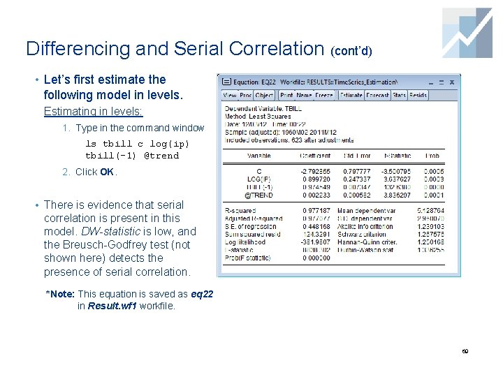
Differencing and Serial Correlation (cont’d) • Let’s first estimate the following model in levels. Estimating in levels: 1. Type in the command window ls tbill c log(ip) tbill(-1) @trend 2. Click OK. • There is evidence that serial correlation is present in this model. DW-statistic is low, and the Breusch-Godfrey test (not shown here) detects the presence of serial correlation. *Note: This equation is saved as eq 22 in Result. wf 1 workfile. 69

Differencing and Serial Correlation (cont’d) • Now let’s estimate the same model in first differences. • Remember that EViews allows you to difference the data very easily by typing d() before the name of the variable or dlog (if you want to take log differences). Estimating the model in first-differences: 1. Type in the command window: ls d(tbill) c dlog(ip) d(tbill(-1))@trend 2. Press Enter. *Note: This equation is saved as eq 23 in Result. wf 1 workfile. 70

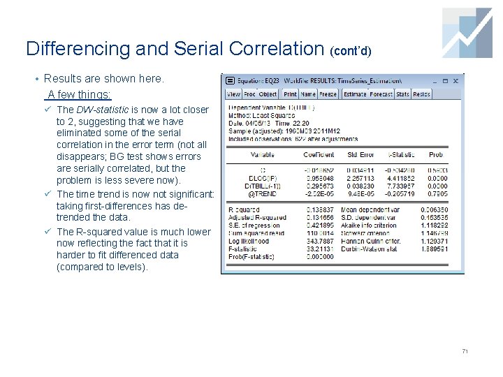
Differencing and Serial Correlation (cont’d) • Results are shown here. A few things: ü The DW-statistic is now a lot closer to 2, suggesting that we have eliminated some of the serial correlation in the error term (not all disappears; BG test shows errors are serially correlated, but the problem is less severe now). ü The time trend is now not significant: taking first-differences has detrended the data. ü The R-squared value is much lower now reflecting the fact that it is harder to fit differenced data (compared to levels). 71

Heteroskedasticity and Autocorrelation In Time Series

Heteroskedasticity and Autocorrelation in Time Series • Nothing rules out the possibility that both heteroskedasticity and serial correlation are present in a regression model. ü Serial correlation has a larger impact on standard errors and efficiency of estimators than heteroskedasticity ü However, heteroskedasticity may be of concern especially in small samples. • In addition, in many financial time series, the conditional variance of the error term depends on past values of the error term. This is also known as autoregressive conditional heteroskedasticity (ARCH). • In this section, we demonstrate the following: ü Testing for heteroskedasticity in time series models ü Testing for ARCH terms ü HAC standard errors 73

Heteroskedasticity and Autocorrelation in Time Series (cont’d) • Testing for Heteroskedasticity in time series data is very similar to cross section data* ü The one caveat is that, when testing for heteroskedasticity, residuals should not be serially correlated. ü Any serial correlation will generally invalidate tests for heteroskedasticity. ü It thus makes sense to test for serial correlation first, correct for serial correlation, and then test for heteroskedasticity. ü Most commonly, you can correct for both heteroskedasticity and autocorrelation of unknown form using the HAC Consistent Covariance (Newey-West). *Note: For heteroskedasticity test on cross-section data see tutorial on Basic Estimation. 74

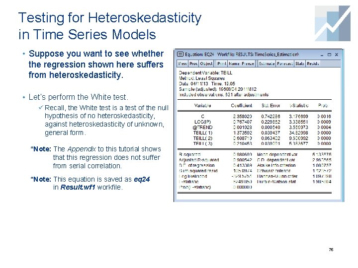
Testing for Heteroskedasticity in Time Series Models • Suppose you want to see whether the regression shown here suffers from heteroskedasticity. • Let’s perform the White test. ü Recall, the White test is a test of the null hypothesis of no heteroskedasticity, against heteroskedasticity of unknown, general form. *Note: The Appendix to this tutorial shows that this regression does not suffer from serial correlation. *Note: This equation is saved as eq 24 in Result. wf 1 workfile. 75

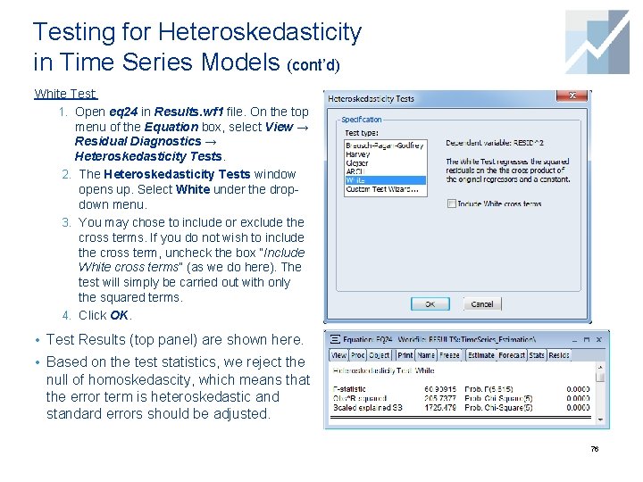
Testing for Heteroskedasticity in Time Series Models (cont’d) White Test: 1. Open eq 24 in Results. wf 1 file. On the top menu of the Equation box, select View → Residual Diagnostics → Heteroskedasticity Tests. 2. The Heteroskedasticity Tests window opens up. Select White under the dropdown menu. 3. You may chose to include or exclude the cross terms. If you do not wish to include the cross term, uncheck the box “Include White cross terms” (as we do here). The test will simply be carried out with only the squared terms. 4. Click OK. • Test Results (top panel) are shown here. • Based on the test statistics, we reject the null of homoskedascity, which means that the error term is heteroskedastic and standard errors should be adjusted. 76

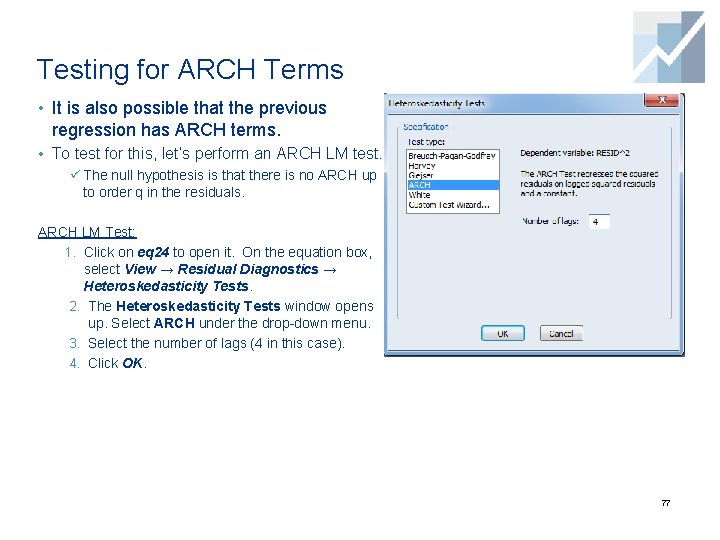
Testing for ARCH Terms • It is also possible that the previous regression has ARCH terms. • To test for this, let’s perform an ARCH LM test. ü The null hypothesis is that there is no ARCH up to order q in the residuals. ARCH LM Test: 1. Click on eq 24 to open it. On the equation box, select View → Residual Diagnostics → Heteroskedasticity Tests. 2. The Heteroskedasticity Tests window opens up. Select ARCH under the drop-down menu. 3. Select the number of lags (4 in this case). 4. Click OK. 77

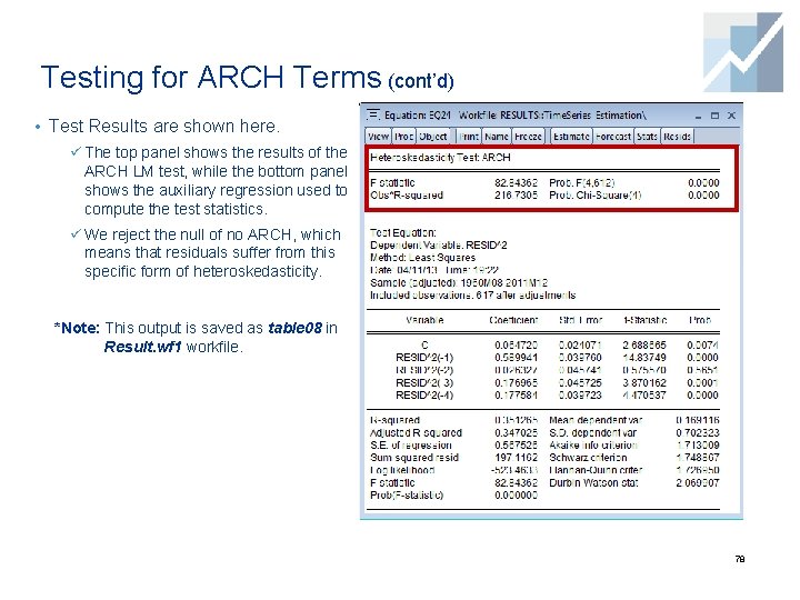
Testing for ARCH Terms (cont’d) • Test Results are shown here. ü The top panel shows the results of the ARCH LM test, while the bottom panel shows the auxiliary regression used to compute the test statistics. ü We reject the null of no ARCH, which means that residuals suffer from this specific form of heteroskedasticity. *Note: This output is saved as table 08 in Result. wf 1 workfile. 78

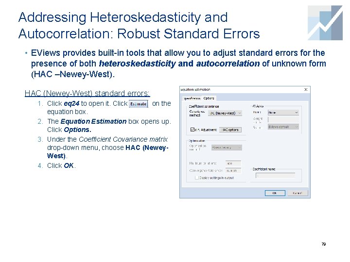
Addressing Heteroskedasticity and Autocorrelation: Robust Standard Errors • EViews provides built-in tools that allow you to adjust standard errors for the presence of both heteroskedasticity and autocorrelation of unknown form (HAC –Newey-West). HAC (Newey-West) standard errors: 1. Click eq 24 to open it. Click on the equation box. 2. The Equation Estimation box opens up. Click Options. 3. Under the Coefficient Covariance matrix drop-down menu, choose HAC (Newey. West). 4. Click OK. 79

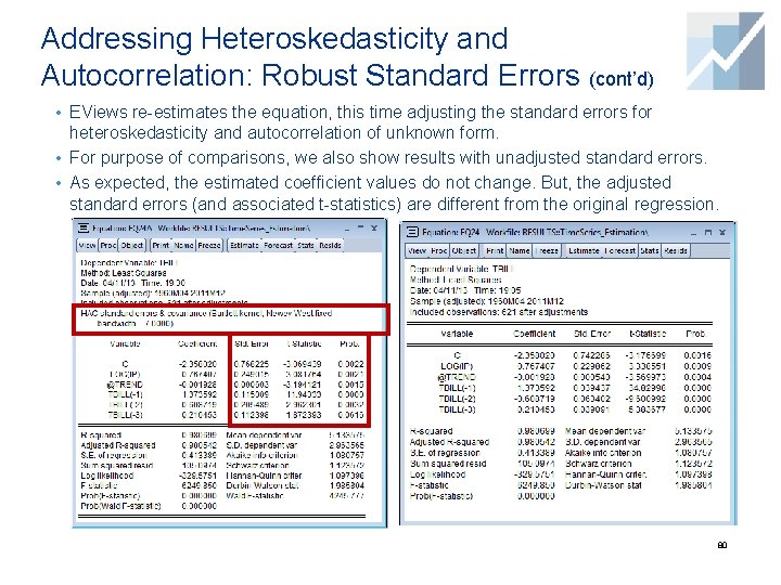
Addressing Heteroskedasticity and Autocorrelation: Robust Standard Errors (cont’d) • EViews re-estimates the equation, this time adjusting the standard errors for heteroskedasticity and autocorrelation of unknown form. • For purpose of comparisons, we also show results with unadjusted standard errors. • As expected, the estimated coefficient values do not change. But, the adjusted standard errors (and associated t-statistics) are different from the original regression. 80