Evaluating precision gain for timber and nontimber attributes

Evaluating precision gain for timber and non-timber attributes via Landsat-based stratification on California’s North Coast Antti Kaartinen, Jeremy Fried & Paul Dunham Other collaborators: Michael Lefsky, Dale Weyermann Dave Portland

Why stratify? Increase precision of inventory estimates by reducing sampling error (std err of estimate/estimate). How does it work? Divides area “population” into strata such that: variability of plots within strata < variability of plots within the population as a whole, and Strata with high variability make up a relatively small proportion of the

Standards of precision Forest Survey Handbook reliability standards: Timberland area: 3% sampling error per million acres Growing stock volume: 10% sampling error per billion cu ft Where sampling error = std error / estimate Are these standards or targets?

Two-phase sampling Phase 1 Collect data for stratification Photo-interpretation for Forest Land Strata (FLS) Phase 2 1/16 of Phase 1 plots are designated field plots Install/measure field plots Efficient strategy for sampling error reduction, but Phase 1 not really cheap

Why evaluate more automated methods? Save time and money? Responsive to national mandate! Standardization could facilitate interpretation Timely- several PIs now 20 years old How current does Phase 1 need to be?

How does FIA stratify elsewhere? Photo-interpretation (PI) in most areas North Central: NLCD + Edge classes Rocky Mountain: AVHRR Northeast: NLCD+5 X 5 pixel moving window filter

PNW’s Stratification Testing Tested 3 LANDSAT-TM based stratification methods Compared with PI & Simple Random Sampling Location criterion: availability of recent PI Antti Kaartinen, Helsinki University Michael Lefsky, multi-institutional Oregon State University strike team: Assembled Dale Weyermann, PNW-FIA, Inv. Reporting & Mapping Paul Dunham, PNW-FIA, Inv. Reporting & Mapping Jeremy Fried, PNW-FIA, Environmental Analysis & Research Dave Azuma, PNW-FIA, Environmental Analysis & Research

Study Area

Stratification sources- all based on TM Existing GIS layers NLCD CALVEG Customized system for generating a new GIS layer FIASCO-TM

NLCD: National Land Cover Dataset Developed at EROS from LANDSAT 5 TM imagery circa 1992 by MRLC Covers lower 48 states Used leaf on/off imagery Built on unsupervised classification, census & National Wetlands Inventory data, and digital terrain models Intended update cycle is 5 -10 years

CALVEG: Classification and Assessment with Landsat of Visible Ecological Groupings Developed by USFS R 5 RSL, Sacramento & CDF LANDSAT-TM data used for life form Other inputs vary by location and include Field observations DEMs Local knowledge Classified polygons include life form, tree cover species and stage of stand development

FIASCO-TM: Forest Inventory and Analysis Stratification with Classification of Thematic Mapper Developed in cooperation with Michael Lefsky, Oregon State University Dept of Forest Science TM scenes trained by a 20% intensity phase 1 PI Semi-automated, supervised classification Uses spectral signature of pixels overlaying a PI point as a basis for classifying other pixels Produces a map of Forest Land Strata

How the class definitions affect the resulting classified image

Image Processing Reprojection Masking Image correction Image mosaic

Landsat scenes from raw images to georeferenced and normalized mosaic

Image Processing Reprojection Masking Image correction Image mosaic Classify/Recode

Recode/cross-walk: NLCD Forest Deciduous Forest Evergreen Forest Mixed Forest Other forest Bare/transitional Shrubland Woody wetland Nonforest Everything else Stratification crosswalks Forest/nonforest (fnf) fnf + other forest (fofnf) Deciduous, evergreen, mixed, other forest, nonforest (DEMON)

Recode/cross-walk: CALVEG 9 cover types Several stand size class, density and species attributes; 100 s of combinations Ultimately aggregated to eight strata Constructed strata 1. 2. 3. 4. 5. 6. 7. 8. non-stocked hardwood low-volume conifer medium-volume conifer high-volume conifer other-forest non-forest unclassified

Image Processing Reprojection Masking Image correction Image mosaic Classify/Recode Post-processing Filtering via clump & sieve

Steps in filtering a classified image file Original classified image Evergreen & mixed forest After clump & sieve After neighborhood analysis Clumps of pixels, that were Smaller than the threshold Value (4 pixels) are removed Majority function in 3*3 pixel window defines a new value for Each ‘empty’ cell Nonstocked forest Deciduous forest Nonproductive forest Nonforest 30 -METER PIXELS

How filtering changes the image

Image Processing Reprojection Masking Image correction Image mosaic Classify/Recode Post-processing Filtering via clump & sieve Edge class generation

Edge classes Edges created around every type Addresses issues of misregistrationinduced incorrect assignments of plots to strata Such incorrectly assigned plots comprise a smaller strata, thus having less impact on overall variance Experimented with edge widths of 2 -4 pixels Edge class effectiveness explored for

Forest / Nonforest with 4 -pixel edge strata Forest Edge Non Forest Edge

DEMON with 4 -pixel strata Evergreen Forest Edge Deciduous Forest Edge Other Forest Edge Non Forest Edge Mixed Forest & Mixed Forest Edge

Table Generation Population estimates & sampling errors for Timberland area Timberland growing stock volume Coarse woody debris volume Area of vegetation cover classes Processed via SAS scripts designed to handle Double sampling Stratified random sampling Simple random sampling Also conventional PI and random (no Phase 1)

Design effect k= after Särndal et al. 1992 k=0. 67 excellent substantial moderate minimal Relative confidence intervals at different levels of statistical efficiency k=1 k=0. 83 k=0. 50 k=0. 25 Variance with stratification Variance with simple random sampling

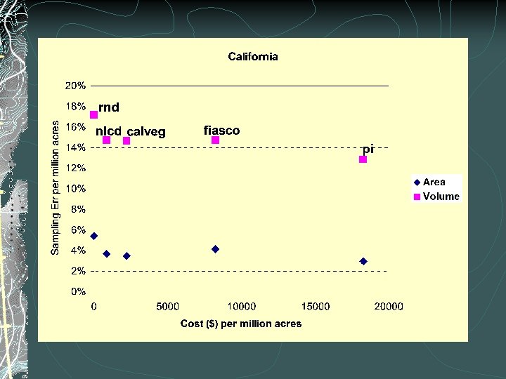
Timberland area Sampling error per 1 million acres

Volume on timberland Sampling error per 1 billion cubic feet

Coarse Woody Debris Sampling error per 1 billion cubic feet

ry vegetatio n cover classes Class 1: (0% shrub cover) Class 2: (0 – 40 % shrub cover) Class 3: ( >= 40 % shrub cover)

Method cost per million acres

PI- advantages Generally high precision Opportunities for ancillary studies Easy to fine tune For areas of interest To fit FIA definitions Opportunities for year-round employment of some data collection staff

NLCD - advantages Could standardize in lower 48 Development costs shared among agencies Pre-rectified/classified imagery huge savings Precision nearly as good as PI for this study area

FIASCO-TM - advantages Easily fine tuned to local conditions/needs Current version gives good precision; may be amenable to improvement Generates a wall-to-wall FLS map which may be useful to some clients

CALVEG - advantages Polygons have many attributes, facilitating customization Data may be useful for other purposes Precision performance good

Caveats Cost comparisons don’t consider value of maps produced incidental to the stratification capacity to conduct ancillary studies self-sufficiency wrt phase 1 production We don’t yet know true costs for NLCD 2000

Sparse forest extension § Forest Cover Thresholds § NLCD = 25% § FIA = 10% § Test aging of phase 1 § Scheduled for Winter 2002 in 4 Central OR counties

Sparse forest extension 1981 and 2001 PI NLCD 1992 FIASCO-TM Built on 1981 PI Built on 2001 PI

Thank you for your patience… Questions? ?