ET 438 b Digital Control and Data Acquisition
ET 438 b Digital Control and Data Acquisition Department of Technology Lesson 12: Analog Signal Conditioning Lesson 12_et 438 b. pptx 1
Learning Objectives After this presentation you will be able to: Ø Design a voltage-to-current interface for a transducer and simulate its operation using commonly available software Ø List the modes of operation of a Wheatstone bridge circuit Ø Explain how Wheatstone bridge resistor values effect linearity and sensitivity Ø Design a signal conditioning circuit for a Wheatstone bridge. Lesson 12_et 438 b. pptx 2
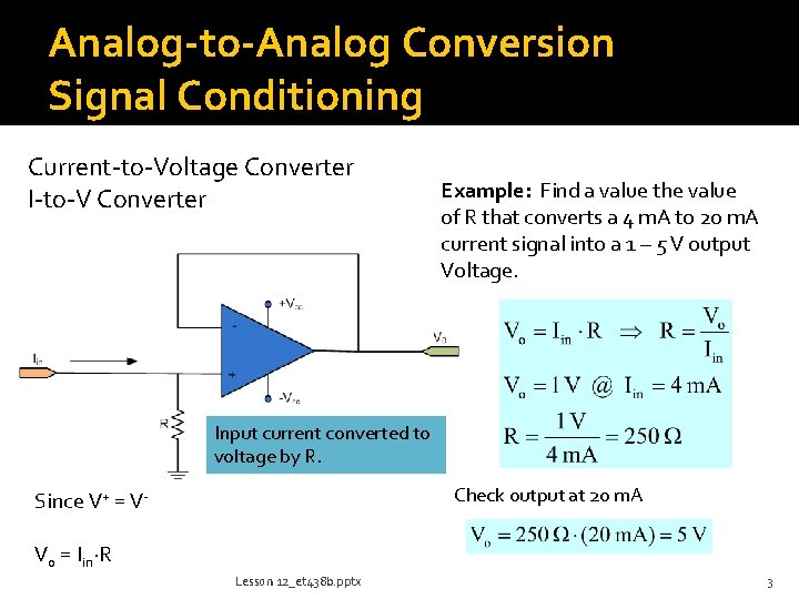
Analog-to-Analog Conversion Signal Conditioning Current-to-Voltage Converter I-to-V Converter Example: Find a value the value of R that converts a 4 m. A to 20 m. A current signal into a 1 – 5 V output Voltage. Input current converted to voltage by R. Check output at 20 m. A Since V+ = VVo = Iin∙R Lesson 12_et 438 b. pptx 3
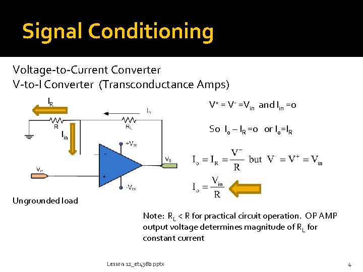
Signal Conditioning Voltage-to-Current Converter V-to-I Converter (Transconductance Amps) IR V+ = V- =Vin and Iin =0 So Io – IR =0 or Io=IR Iin Ungrounded load Note: RL < R for practical circuit operation. OP AMP output voltage determines magnitude of RL for constant current Lesson 12_et 438 b. pptx 4
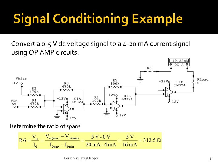
Signal Conditioning Example Convert a 0 -5 V dc voltage signal to a 4 -20 m. A current signal using OP AMP circuits. Determine the ratio of spans Lesson 12_et 438 b. pptx 5
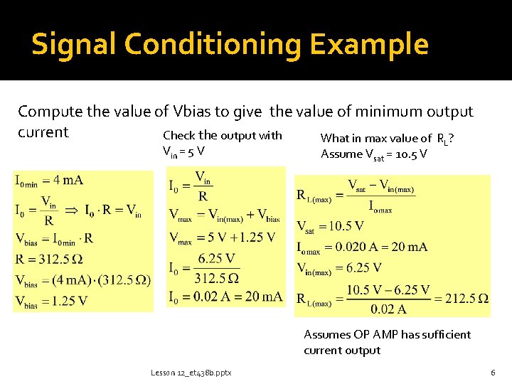
Signal Conditioning Example Compute the value of Vbias to give the value of minimum output current Check the output with What in max value of R ? Vin = 5 V Assume Vsat = 10. 5 V L Assumes OP AMP has sufficient current output Lesson 12_et 438 b. pptx 6
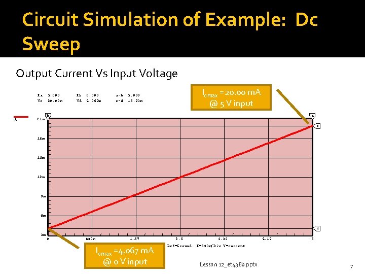
Circuit Simulation of Example: Dc Sweep Output Current Vs Input Voltage Xa: 5. 000 Yc: 20. 00 m A 21 m Xb: 0. 000 Yd: 4. 067 m Iomax =20. 00 m. A @ 5 V input a-b: 5. 000 c-d: 15. 93 m b a c 18 m 15 m 12 m 9 m 6 m d 3 m 0 833 m 1. 67 Iomax =4. 067 m. A @ 0 V input 2. 5 Ref=Ground 3. 33 4. 17 5 X=833 m/Div Y=current Lesson 12_et 438 b. pptx 7
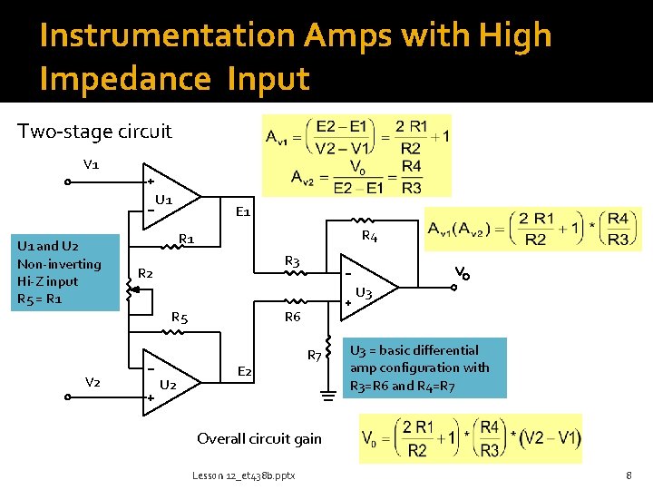
Instrumentation Amps with High Impedance Input Two-stage circuit V 1 U 1 and U 2 Non-inverting Hi-Z input R 5 = R 1 E 1 R 4 R 1 R 3 R 2 U 3 R 5 V 2 U 2 R 6 E 2 R 7 U 3 = basic differential amp configuration with R 3=R 6 and R 4=R 7 Overall circuit gain Lesson 12_et 438 b. pptx 8
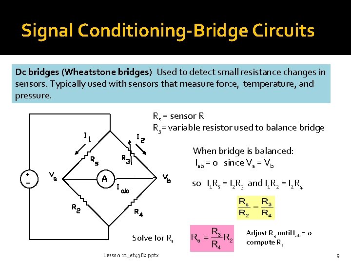
Signal Conditioning-Bridge Circuits Dc bridges (Wheatstone bridges) Used to detect small resistance changes in sensors. Typically used with sensors that measure force, temperature, and pressure. Rs = sensor R R 3= variable resistor used to balance bridge When bridge is balanced: Iab = 0 since Va = Vb so I 1 Rs = I 2 R 3 and I 1 R 2 = I 2 R 4 Solve for Rs Lesson 12_et 438 b. pptx Adjust R 3 until Iab = 0 compute Rs 9
Bridge Use Methods There are two operating modes for a dc bridge: balanced (null) and unbalanced Null Mode - adjust R 3 variable resistor until Iab = 0. Need automatic nulling circuit for automatic operation. Unbalanced Mode - insert sensor and null bridge for sensor measurement. When initial value of sensor changes measure difference in voltage. Bridge only balanced at one point Lesson 12_et 438 b. pptx 10
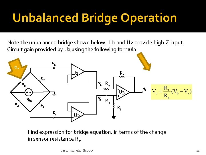
Unbalanced Bridge Operation Note the unbalanced bridge shown below. U 1 and U 2 provide high-Z input. Circuit gain provided by U 3 using the following formula. Rs U 1 Rf Ra U 3 Ra Rf U 2 Find expression for bridge equation. in terms of the change in sensor resistance Rs. Lesson 12_et 438 b. pptx 11
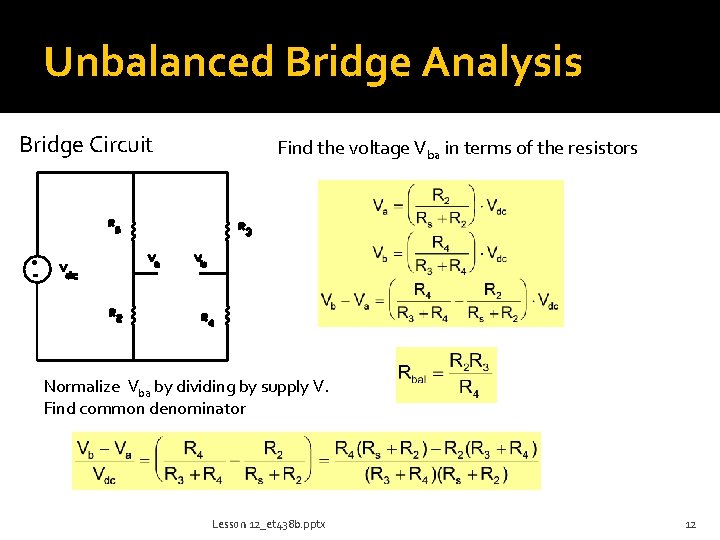
Unbalanced Bridge Analysis Bridge Circuit Find the voltage Vba in terms of the resistors Normalize Vba by dividing by supply V. Find common denominator Lesson 12_et 438 b. pptx 12
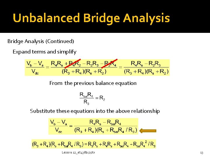
Unbalanced Bridge Analysis (Continued) Expand terms and simplify From the previous balance equation Substitute these equations into the above relationship Lesson 12_et 438 b. pptx 13
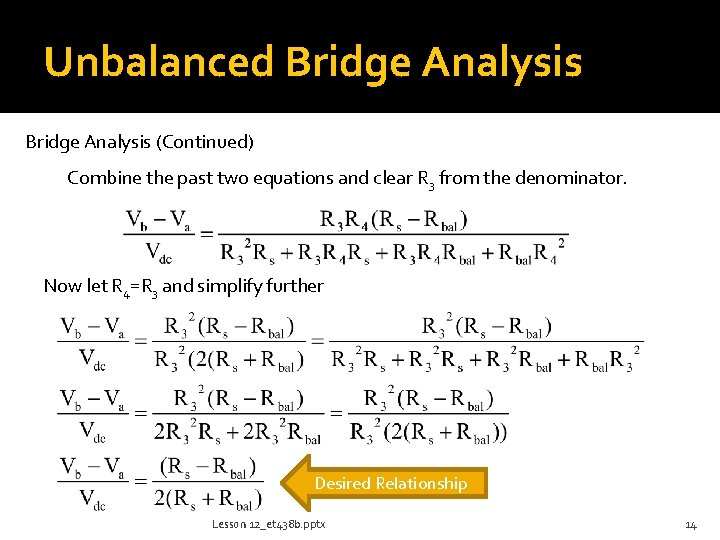
Unbalanced Bridge Analysis (Continued) Combine the past two equations and clear R 3 from the denominator. Now let R 4=R 3 and simplify further Desired Relationship Lesson 12_et 438 b. pptx 14
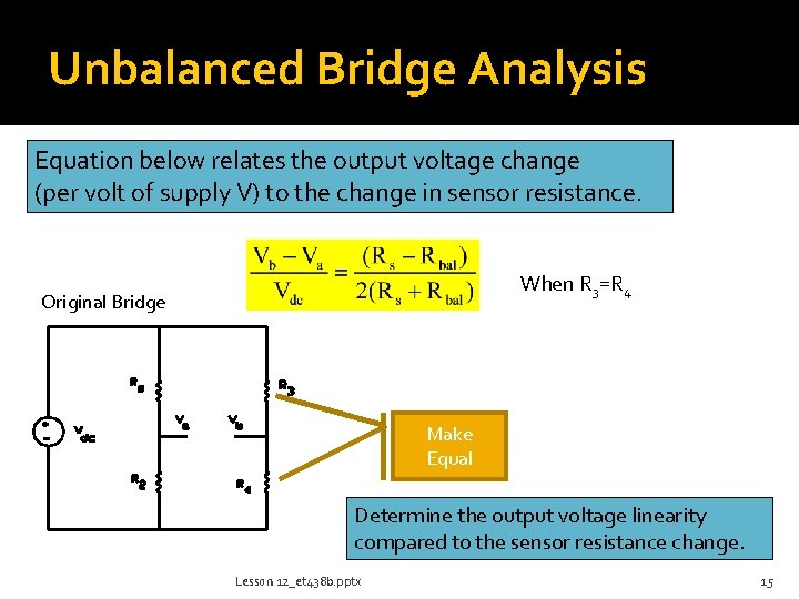
Unbalanced Bridge Analysis Equation below relates the output voltage change (per volt of supply V) to the change in sensor resistance. When R 3=R 4 Original Bridge Make Equal Determine the output voltage linearity compared to the sensor resistance change. Lesson 12_et 438 b. pptx 15
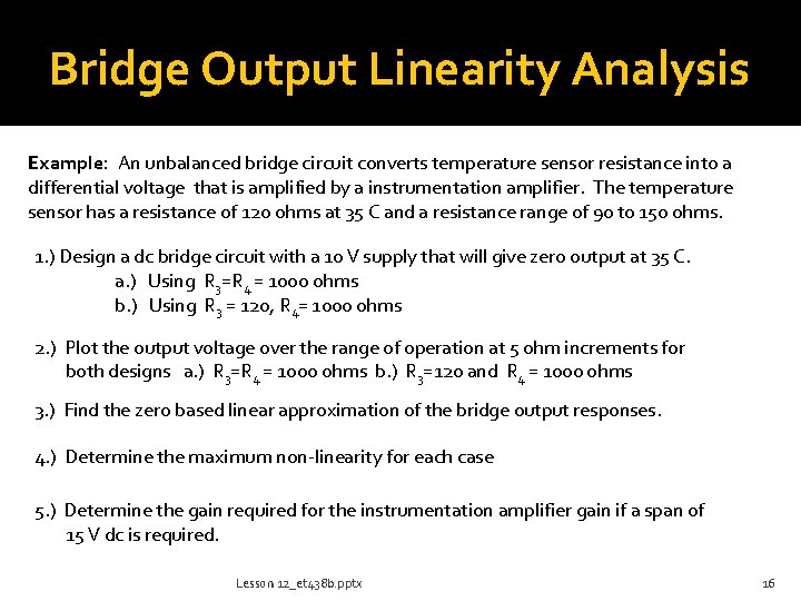
Bridge Output Linearity Analysis Example: An unbalanced bridge circuit converts temperature sensor resistance into a differential voltage that is amplified by a instrumentation amplifier. The temperature sensor has a resistance of 120 ohms at 35 C and a resistance range of 90 to 150 ohms. 1. ) Design a dc bridge circuit with a 10 V supply that will give zero output at 35 C. a. ) Using R 3=R 4 = 1000 ohms b. ) Using R 3 = 120, R 4= 1000 ohms 2. ) Plot the output voltage over the range of operation at 5 ohm increments for both designs a. ) R 3=R 4 = 1000 ohms b. ) R 3=120 and R 4 = 1000 ohms 3. ) Find the zero based linear approximation of the bridge output responses. 4. ) Determine the maximum non-linearity for each case 5. ) Determine the gain required for the instrumentation amplifier gain if a span of 15 V dc is required. Lesson 12_et 438 b. pptx 16
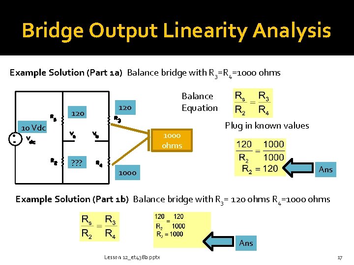
Bridge Output Linearity Analysis Example Solution (Part 1 a) Balance bridge with R 3=R 4=1000 ohms 120 10 Vdc Balance Equation 1000 ohms ? ? ? Plug in known values Ans 1000 Example Solution (Part 1 b) Balance bridge with R 3= 120 ohms R 4=1000 ohms Ans Lesson 12_et 438 b. pptx 17
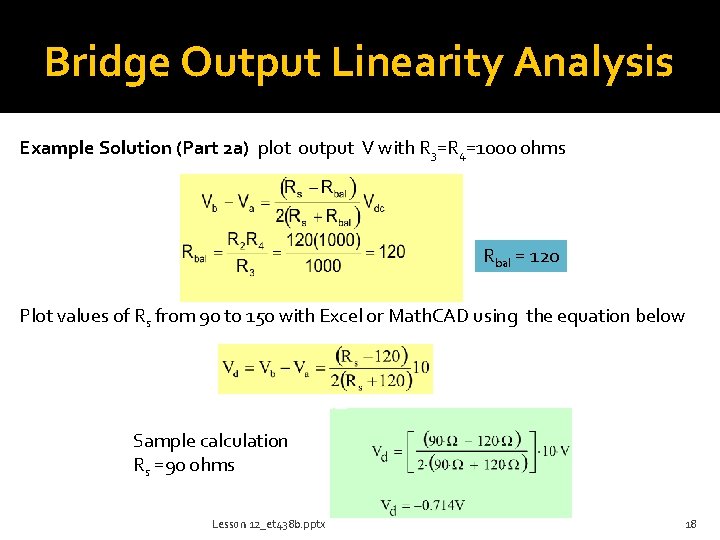
Bridge Output Linearity Analysis Example Solution (Part 2 a) plot output V with R 3=R 4=1000 ohms Rbal = 120 Plot values of Rs from 90 to 150 with Excel or Math. CAD using the equation below Sample calculation Rs =90 ohms Lesson 12_et 438 b. pptx 18
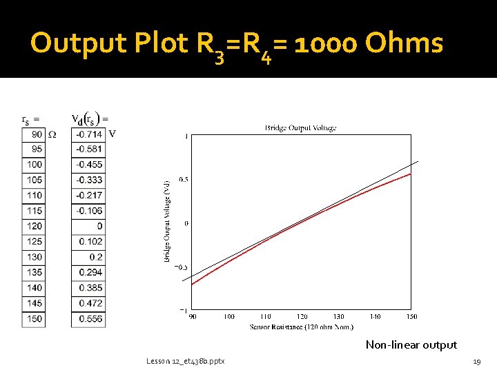
Output Plot R 3=R 4= 1000 Ohms Non-linear output Lesson 12_et 438 b. pptx 19
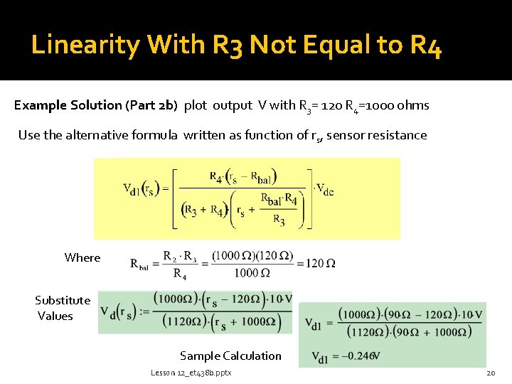
Linearity With R 3 Not Equal to R 4 Example Solution (Part 2 b) plot output V with R 3= 120 R 4=1000 ohms Use the alternative formula written as function of rs, sensor resistance Where Substitute Values Sample Calculation Lesson 12_et 438 b. pptx 20
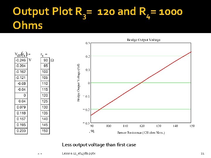
Output Plot R 3= 120 and R 4= 1000 Ohms Less output voltage than first case Lesson 12_et 438 b. pptx 21
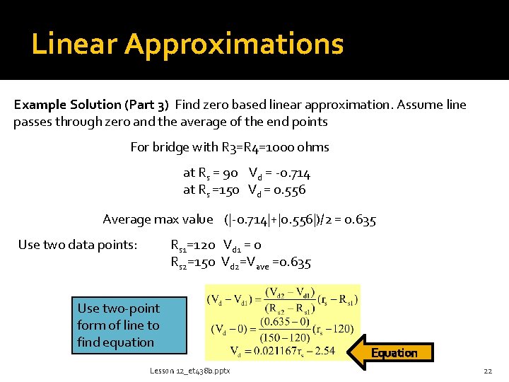
Linear Approximations Example Solution (Part 3) Find zero based linear approximation. Assume line passes through zero and the average of the end points For bridge with R 3=R 4=1000 ohms at Rs = 90 Vd = -0. 714 at Rs =150 Vd = 0. 556 Average max value (|-0. 714|+|0. 556|)/2 = 0. 635 Use two data points: Rs 1=120 Vd 1 = 0 Rs 2=150 Vd 2=Vave =0. 635 Use two-point form of line to find equation Lesson 12_et 438 b. pptx Equation 22
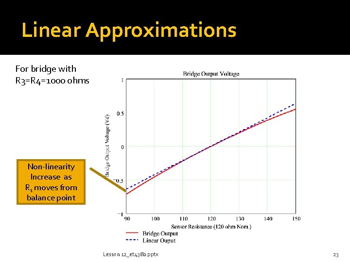
Linear Approximations For bridge with R 3=R 4=1000 ohms Non-linearity Increase as Rs moves from balance point Lesson 12_et 438 b. pptx 23
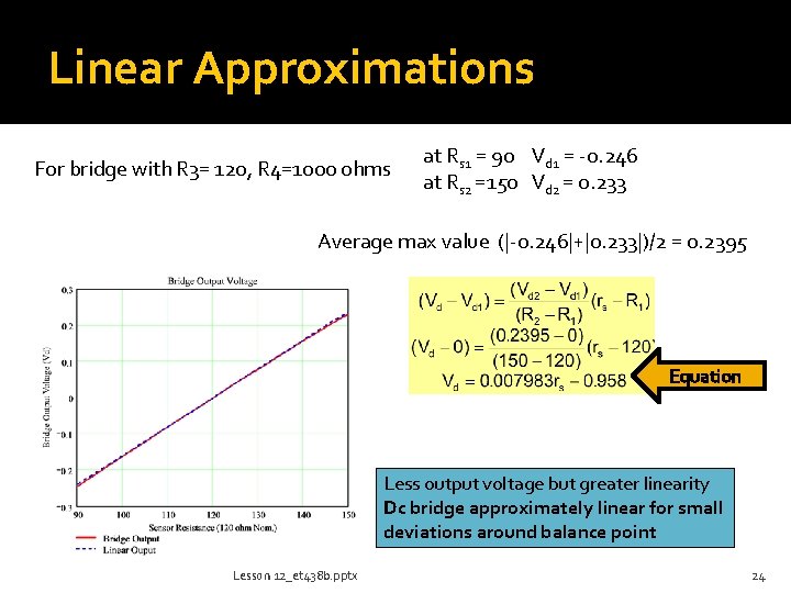
Linear Approximations For bridge with R 3= 120, R 4=1000 ohms at Rs 1 = 90 Vd 1 = -0. 246 at Rs 2 =150 Vd 2 = 0. 233 Average max value (|-0. 246|+|0. 233|)/2 = 0. 2395 Equation Less output voltage but greater linearity Dc bridge approximately linear for small deviations around balance point Lesson 12_et 438 b. pptx 24
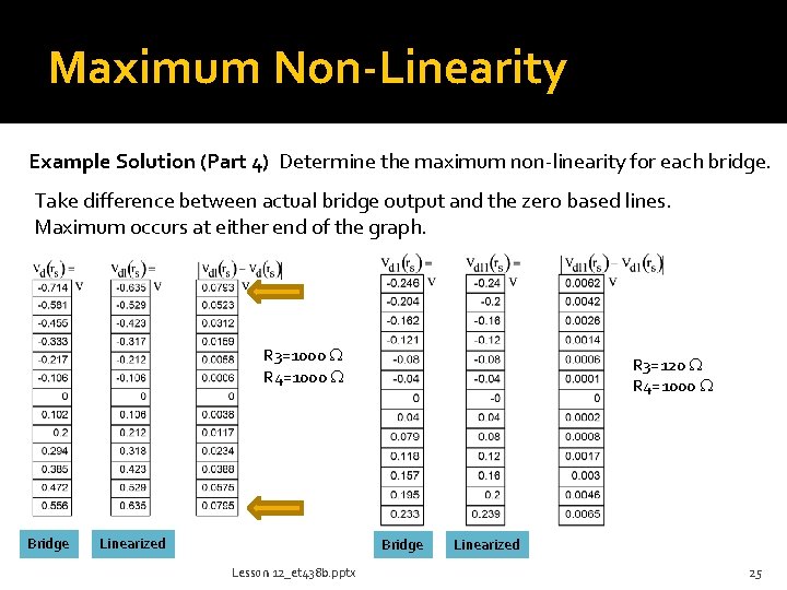
Maximum Non-Linearity Example Solution (Part 4) Determine the maximum non-linearity for each bridge. Take difference between actual bridge output and the zero based lines. Maximum occurs at either end of the graph. R 3=1000 W R 4=1000 W Bridge Linearized R 3=120 W R 4=1000 W Bridge Lesson 12_et 438 b. pptx Linearized 25
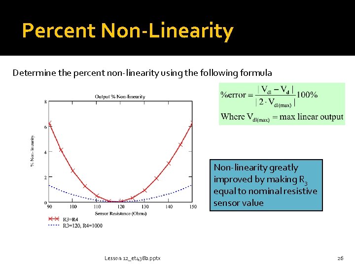
Percent Non-Linearity Determine the percent non-linearity using the following formula Non-linearity greatly improved by making R 3 equal to nominal resistive sensor value Lesson 12_et 438 b. pptx 26
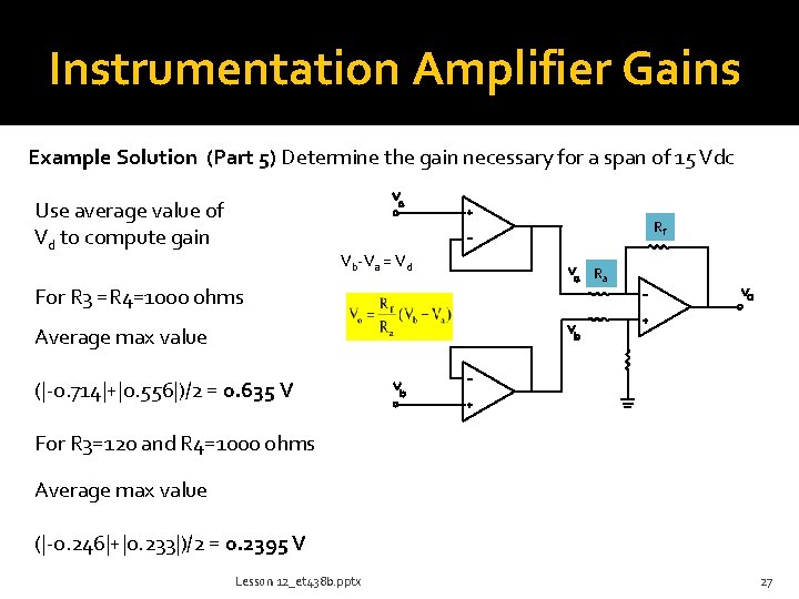
Instrumentation Amplifier Gains Example Solution (Part 5) Determine the gain necessary for a span of 15 Vdc Use average value of Vd to compute gain Rf Vb-Va = Vd For R 3 =R 4=1000 ohms Ra Average max value (|-0. 714|+|0. 556|)/2 = 0. 635 V For R 3=120 and R 4=1000 ohms Average max value (|-0. 246|+|0. 233|)/2 = 0. 2395 V Lesson 12_et 438 b. pptx 27
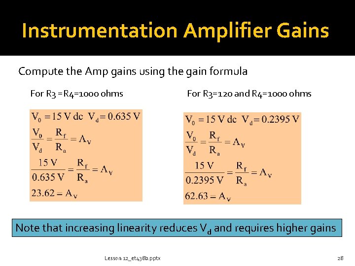
Instrumentation Amplifier Gains Compute the Amp gains using the gain formula For R 3 =R 4=1000 ohms For R 3=120 and R 4=1000 ohms Note that increasing linearity reduces Vd and requires higher gains Lesson 12_et 438 b. pptx 28
End Lesson 12: Analog Signal Conditioning ET 438 b Digital Control and Data Acquisition Department of Technology Lesson 12_et 438 b. pptx 29
- Slides: 29