Estimation Value of Ambiguity in Ensemble Forecasts Tony

Estimation & Value of Ambiguity in Ensemble Forecasts Tony Eckel National Weather Service Office of Science and Technology, Silver Spring, MD Mark Allen Air Force Weather Agency, Omaha, NE Eckel, F. A. , M. S. Allen, and M. C. Sittel, 2012: Estimation of ambiguity in ensemble forecasts. Weather and Forecasting, in press. Allen, M. S. and F. A. Eckel, 2012: Value from ambiguity in ensemble forecasts. Weather and Forecasting, in press.

Part I. Estimation of Ambiguity

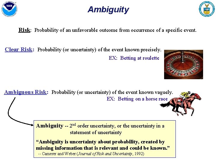
Ambiguity Risk: Probability of an unfavorable outcome from occurrence of a specific event. Clear Risk: Probability (or uncertainty) of the event known precisely. EX: Betting at roulette Ambiguous Risk: Probability (or uncertainty) of the event known vaguely. EX: Betting on a horse race Ambiguity -- 2 nd order uncertainty, or the uncertainty in a statement of uncertainty “Ambiguity is uncertainty about probability, created by missing information that is relevant and could be known. ” -- Camerer and Weber (Journal of Risk and Uncertainty, 1992)

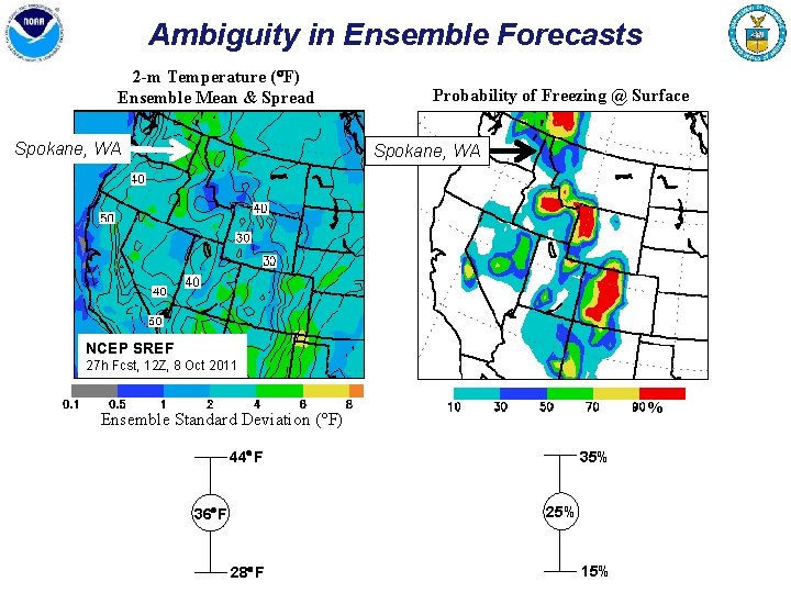
Ambiguity in Ensemble Forecasts 2 -m Temperature ( F) Ensemble Mean & Spread Spokane, WA Probability of Freezing @ Surface Spokane, WA NCEP SREF 27 h Fcst, 12 Z, 8 Oct 2011 % Ensemble Standard Deviation ( F) 35% 44 F 25% 36 F 28 F 15%

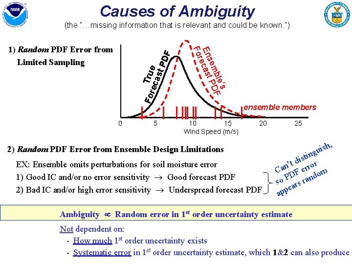
Causes of Ambiguity (the “…missing information that is relevant and could be known. ”) F For True eca st P D 0 5 ’s ble F sem PD En ecast For 1) Random PDF Error from Limited Sampling ensemble members 10 15 Wind Speed (m/s) 20 2) Random PDF Error from Ensemble Design Limitations EX: Ensemble omits perturbations for soil moisture error 1) Good IC and/or no error sensitivity Good forecast PDF 2) Bad IC and/or high error sensitivity Underspread forecast PDF 25 sh, i u ting s i t d ror ’ n Ca F er om D d so P ars ran e app Ambiguity Random error in 1 st order uncertainty estimate Not dependent on: - How much 1 st order uncertainty exists - Systematic error in 1 st order uncertainty estimate, which 1&2 can also produce

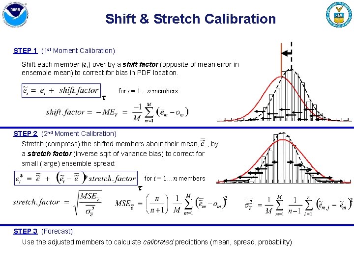
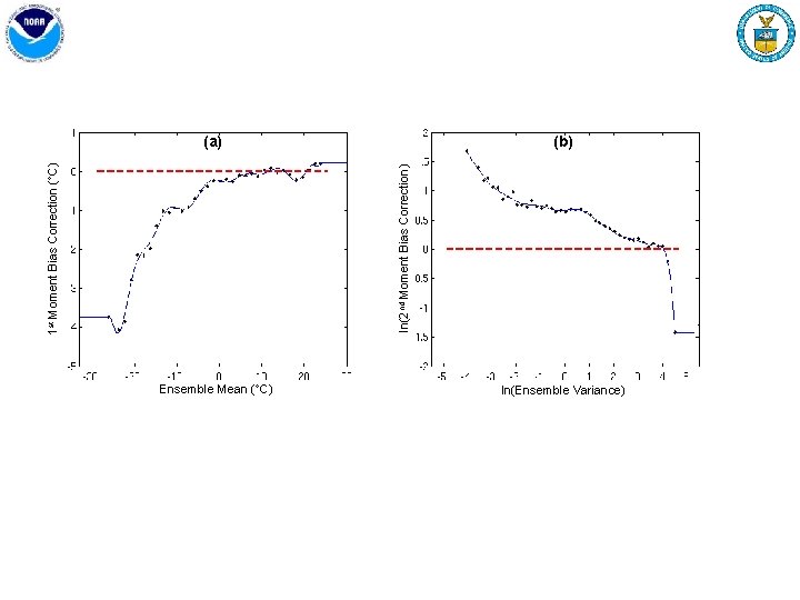
Shift & Stretch Calibration STEP 1 (1 st Moment Calibration) Shift each member (ei) over by a shift factor (opposite of mean error in ensemble mean) to correct for bias in PDF location. for i = 1…n members STEP 2 (2 nd Moment Calibration) Stretch (compress) the shifted members about their mean, , by a stretch factor (inverse sqrt of variance bias) to correct for small (large) ensemble spread: for i = 1…n members STEP 3 (Forecast) Use the adjusted members to calculate calibrated predictions (mean, spread, probability)

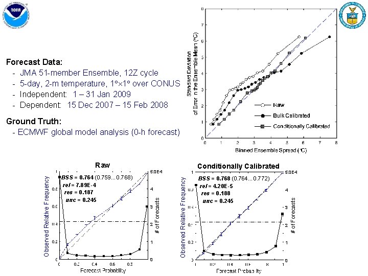
Forecast Data: - JMA 51 -member Ensemble, 12 Z cycle - 5 -day, 2 -m temperature, 1 1 over CONUS - Independent: 1 – 31 Jan 2009 - Dependent: 15 Dec 2007 – 15 Feb 2008 Ground Truth: - ECMWF global model analysis (0 -h forecast) 3 2 1 0 BSS = 0. 768 (0. 764… 0. 772) rel = 4. 20 E-5 res = 0. 188 unc = 0. 245 5. 0 E 4 4 3 2 1 0 # of Forecasts 4 Observed Relative Frequency BSS = 0. 764 (0. 759… 0. 768) rel = 7. 89 E-4 res = 0. 187 unc = 0. 245 Conditionally Calibrated 5. 0 E 4 # of Forecasts Observed Relative Frequency Raw

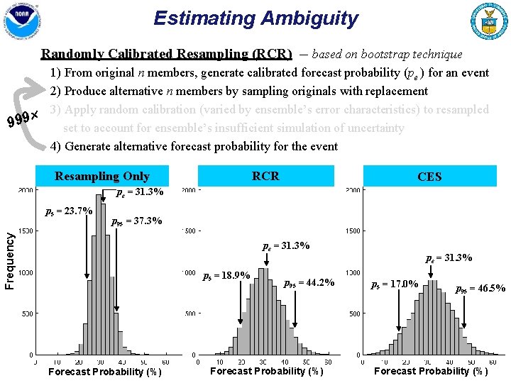
Estimating Ambiguity Randomly Calibrated Resampling (RCR) -- based on bootstrap technique 1) From original n members, generate calibrated forecast probability (pe ) for an event 2) Produce alternative n members by sampling originals with replacement 3) Apply random calibration (varied by ensemble’s error characteristics) to resampled 999 set to account for ensemble’s insufficient simulation of uncertainty 4) Generate alternative forecast probability for the event Resampling Only RCR CES pe = 31. 3% p 95 = 37. 3% Frequency p 5 = 23. 7% pe = 31. 3% p 5 = 18. 9% Forecast Probability (%) pe = 31. 3% p 5 = 16. 5% p 95 = 44. 2% Forecast Probability (%) p 5 = 17. 0% p 95 = 46. 5% Forecast Probability (%)

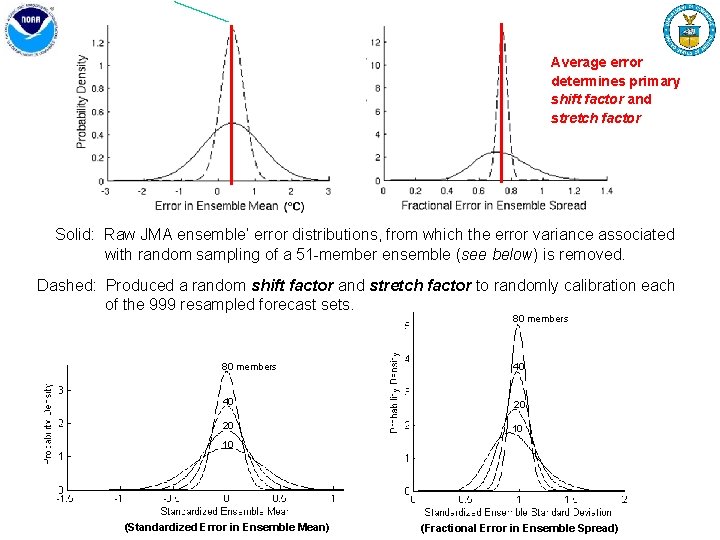
Average error determines primary shift factor and stretch factor Solid: Raw JMA ensemble’ error distributions, from which the error variance associated with random sampling of a 51 -member ensemble (see below) is removed. Dashed: Produced a random shift factor and stretch factor to randomly calibration each of the 999 resampled forecast sets. 80 members 40 40 20 20 10 10 (Standardized Error in Ensemble Mean) (Fractional Error in Ensemble Spread)

Part II. Application of Ambiguity

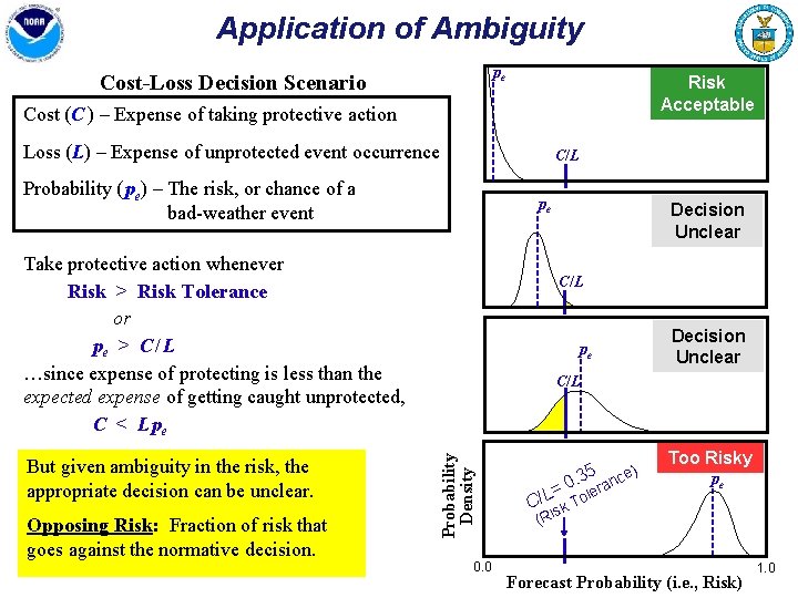
Application of Ambiguity pe Cost-Loss Decision Scenario Risk Acceptable Cost (C ) – Expense of taking protective action Loss (L) – Expense of unprotected event occurrence C/L Probability ( pe) – The risk, or chance of a bad-weather event pe Take protective action whenever Risk > Risk Tolerance or pe > C / L …since expense of protecting is less than the expected expense of getting caught unprotected, C < L pe Opposing Risk: Fraction of risk that goes against the normative decision. C/L Decision Unclear pe C/L Probability Density But given ambiguity in the risk, the appropriate decision can be unclear. Decision Unclear 0. 0 . 35 0 ra /L= Tole n ce) Too Risky pe C sk Ri ( Forecast Probability (i. e. , Risk) 1. 0

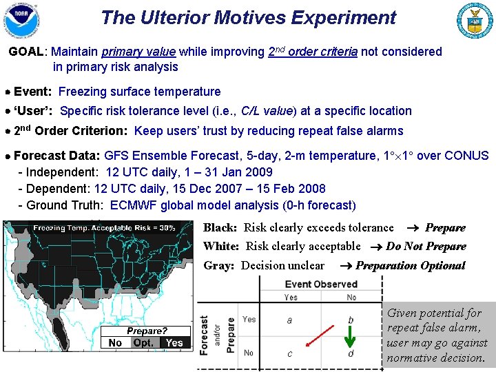
The Ulterior Motives Experiment GOAL: Maintain primary value while improving 2 nd order criteria not considered in primary risk analysis Event: Freezing surface temperature ‘User’: Specific risk tolerance level (i. e. , C/L value) at a specific location 2 nd Order Criterion: Keep users’ trust by reducing repeat false alarms Forecast Data: GFS Ensemble Forecast, 5 -day, 2 -m temperature, 1 1 over CONUS - Independent: 12 UTC daily, 1 – 31 Jan 2009 - Dependent: 12 UTC daily, 15 Dec 2007 – 15 Feb 2008 - Ground Truth: ECMWF global model analysis (0 -h forecast) Black: Risk clearly exceeds tolerance Prepare White: Risk clearly acceptable Do Not Prepare Gray: Decision unclear Preparation Optional Given potential for repeat false alarm, user may go against normative decision.

8 User Behaviors Behavior Name Behavior Description

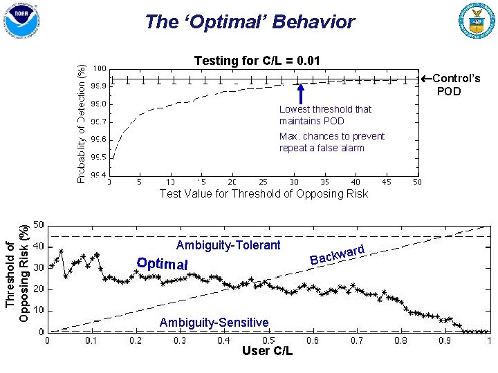
The ‘Optimal’ Behavior Testing for C/L = 0. 01 Control’s POD Lowest threshold that maintains POD Max. chances to prevent repeat a false alarm Threshold of Opposing Risk (%) Test Value for Threshold of Opposing Risk Ambiguity-Tolerant Optimal Ambiguity-Sensitive User C/L ard Backw

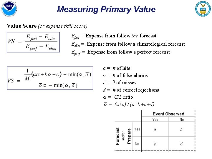
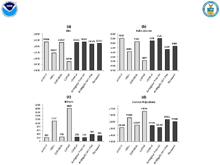
Measuring Primary Value Score (or expense skill score) Efcst = Expense from follow the forecast Eclim = Expense from follow a climatological forecast Eperf = Expense from follow a perfect forecast a = # of hits b = # of false alarms c = # of misses d = # of correct rejections a = C/L ratio = (a+c) / (a+b+c+d)

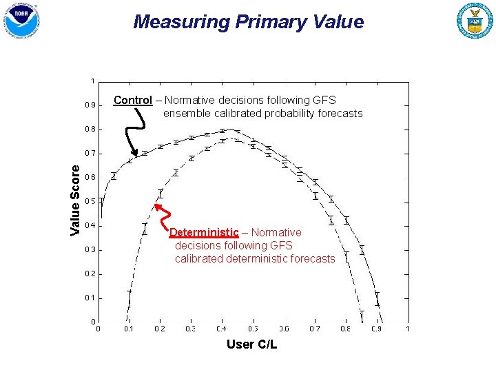
Measuring Primary Value Score Control – Normative decisions following GFS ensemble calibrated probability forecasts Deterministic – Normative decisions following GFS calibrated deterministic forecasts User C/L

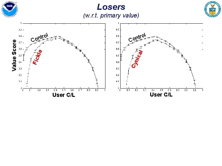
Losers ol r t n Co l nic al kle tro n o C Cy Fic Value Score (w. r. t. primary value) User C/L

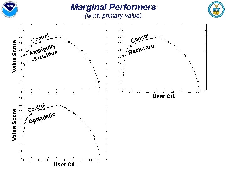
Marginal Performers Value Score (w. r. t. primary value) trol n o C ity u g i b Am sitive -Sen ol r t n Co ard w k Bac Value Score User C/L ol tr Con mis i t p O tic User C/L

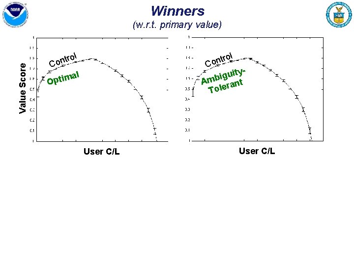
Winners Value Score (w. r. t. primary value) ol r t n Co ityu g i Amb rant Tole trol n o C mal i t p O User C/L

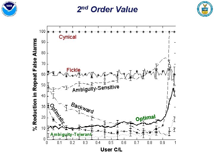
Cynical Fickle e sitiv Ambiguity-Sen Bac kwa rd l Optima ic ist tim Op % Reduction in Repeat False Alarms 2 nd Order Value Ambiguity-Tolerant User C/L

Conclusions Ambiguity in ensemble forecasts can be effectively estimated Users can benefit from ambiguity information through improvement of 2 nd order criteria, but that requires lots of creativity

Backup Slides

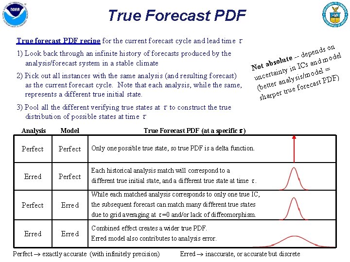
True Forecast PDF True forecast PDF recipe for the current forecast cycle and lead time 1) Look back through an infinite history of forecasts produced by the analysis/forecast system in a stable climate 2) Pick out all instances with the same analysis (and resulting forecast) as the current forecast cycle. Note that each analysis, while the same, represents a different true initial state. 3) Pool all the different verifying true states at to construct the true distribution of possible states at time s on d n e p -- de del o e t m u l d an bso Not a nty in ICs el = tai od uncer nalysis/m PDF) t a s r a e c fore (bett e u r t er sharp True Forecast PDF (at a specific ) Analysis Model Perfect Only one possible true state, so true PDF is a delta function. Erred Perfect Each historical analysis match will correspond to a different true initial state, and a different true state at time . Perfect Erred While each matched analysis corresponds to only one true IC, the subsequent forecast can match many different true states due to grid averaging at =0 and/or lack of diffeomorphism. Erred Combined effect creates a wider true PDF. Erred model also contributes to analysis error. Perfect exactly accurate (with infinitely precision) Erred inaccurate, or accurate but discrete

ln(2 nd Moment Bias Correction) 1 st Moment Bias Correction ( C) (a) Ensemble Mean ( C) (b) ln(Ensemble Variance)

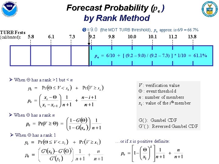
Forecast Probability (pe ) by Rank Method TURB Fcsts 5. 8 (calibrated): 6. 1 7. 3 = 9. 0 (the MDT TURB threshold), pe approx. is 6/9 = 66. 7% 9. 2 9. 8 10. 0 10. 1 11. 2 13. 8 pe = 6/10 + [ (9. 2 – 9. 0) / (9. 2 – 7. 3) ] * 1/10 = 61. 1% Ø When has a rank >1 but < n V : verification value : event threshold n : number of members xi : value of the ith member Ø When has a rank n G( ): Gumbel CDF G’( ): Reversed Gumbel CDF Ø When has a rank 1 …or if x is positive definite:

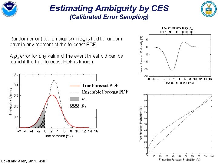
Estimating Ambiguity by CES (Calibrated Error Sampling) Random error (i. e. , ambiguity) in pe is tied to random error in any moment of the forecast PDF. A pe error for any value of the event threshold can be found if the true forecast PDF is known. Eckel and Allen, 2011, WAF

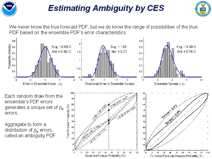
Estimating Ambiguity by CES We never know the true forecast PDF, but we do know the range of possibilities of the true PDF based on the ensemble PDF’s error characteristics: Each random draw from the ensemble’s PDF errors generates a unique set of pe errors. Aggregate to form a distribution of pe errors, called an ambiguity PDF. C 0 ad re Sp d ea r Sp = 2. C 0 = 6.

Estimating Ambiguity by CES Ambiguity PDFs follow the beta distribution.

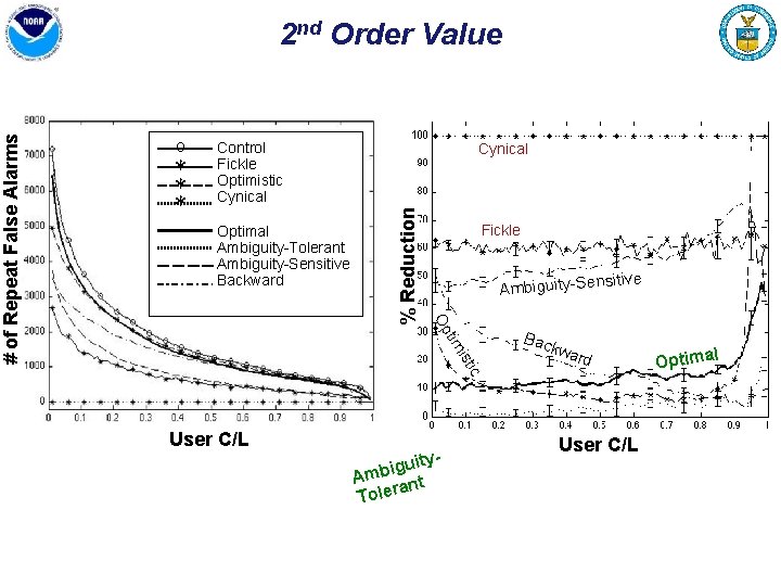
* * * Control Fickle Optimistic Cynical Optimal Ambiguity-Tolerant Ambiguity-Sensitive Backward Cynical % Reduction o Fickle sitive Ambiguity-Sen Bac kwa rd ic ist tim Op # of Repeat False Alarms 2 nd Order Value User C/L uityg i b Am rant e l o T User C/L l Optima

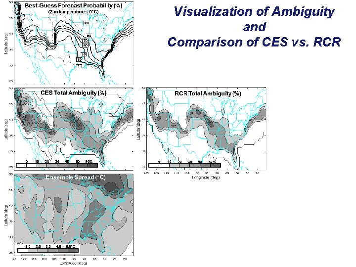
Visualization of Ambiguity and Comparison of CES vs. RCR