Estimation of linear observation impact and its applications
![Estimation of linear observation impact and its applications Toshiyuki Ishibashi MRI/JMA, Japan ishibasi[AT]mri-jma. go.](https://slidetodoc.com/presentation_image_h2/2872cc53742c33271132970749d609b6/image-1.jpg "Estimation of linear observation impact and its applications Toshiyuki Ishibashi MRI/JMA, Japan ishibasi[AT]mri-jma. go.")
Estimation of linear observation impact and its applications Toshiyuki Ishibashi MRI/JMA, Japan ishibasi[AT]mri-jma. go. jp * MRI: Meteorological Research Institute. **JMA: Japan Meteorological Agency.
-based estimation l TL (Tangent")
Contents 1. Observation impact estimation l Definitions l AD (Adjoint)-based estimation l TL (Tangent linear)-based estimation 2. Error covariance matrix optimization l Optimization and observation impact l AD-based optimization 3. Analysis error estimation l Unification of all usable information 4. Summary

1. Observation impact estimation

Observation impact Two definitions l Basic definition p The observation impact is defined as “the variations of analyses and forecasts caused by changes of observation data”. l Non-linear observation impact p This is the observation impact that has no limitations on the changes of observation data, so the changes includes perturbations in observation data values, and additions of observation datasets. p Estimation methods: ü OSE (observing system experiment). l Linear observation impact p This is the observation impact that has an limitation on the changes of observation data, that is Kalman gain is invariant. p Estimation methods are ü AD-based method l Langland Baker (2004), Errico (2007), Cardinali (2009), Tremolet (2008) ü DFS l Cardinali et al (2004), Desroziers et al (2005) ü TL-based method l Ishibashi (2011) These two observation impacts are different quantities, so, in general, they cannot work as a proxy for each other.

Variances of functions of analyses l In linear analyses, we consider four independent variables, a background field xb , observations y, a background error covariance matrix B, and an observation error covariance matrix R. l We can evaluate impacts of each variable.
 Tellus 6")
AD-based estimation Langland Baker (2004) Tellus 6

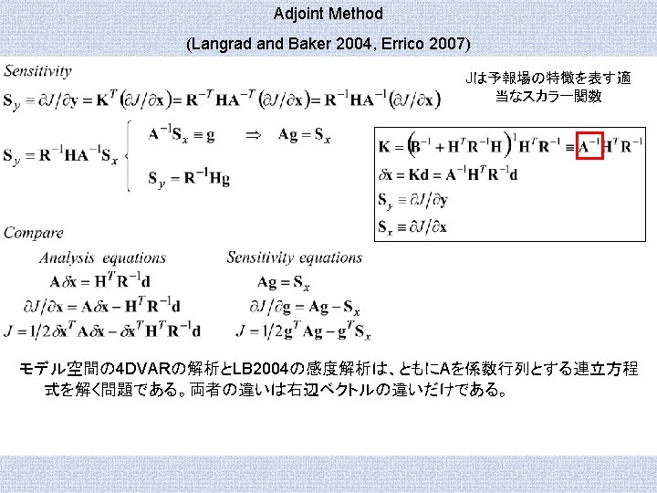
AD-based estimation The formulation of AD-based method under TL approximation: • Definition of a scalar function F of a forecast error vector: C: norm define matrix M: tangent linear model • ef: forecast error vector Variation of F caused by an analysis eb: background error δx: analysis increment Each term is a inner product between the first-order quantities of TL approximation. • For example, a linear observation impact of a dataset P is calculated as follows;

AD-based estimation in JMA global 4 D-Var δJ DRY l JMA global 4 D-Var l Evaluation periods are: Summer: Aug 2010, Winter: Jan 2010. * 00 UTC analyses only. l Using dry total energy norm. l Forecast error evaluation time is 15 hours.

AD-based estimation in JMA global 4 D-Var δJ DRY

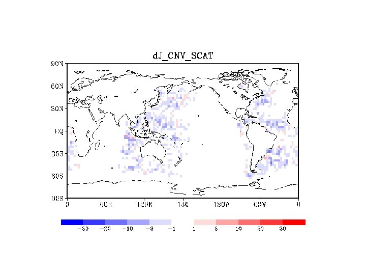
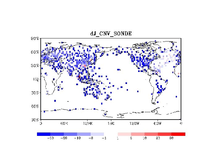
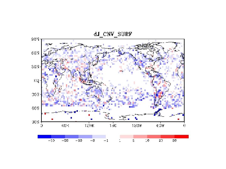
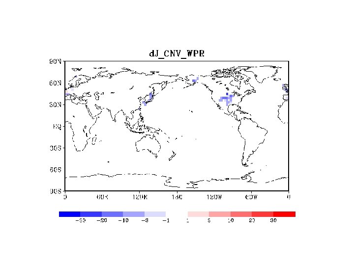
Vertically integrated contribution map

PDF SONDE AMSU-A l About a half observations decrease forecast errors, and the other increase them. l The slope of PDF is different between these data. SONDE is shallower than AMSU-A. l We can guess that the gradient of the slope depends on R and B settings and real information amount of data.

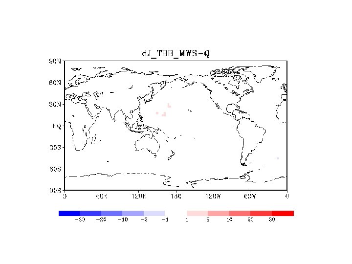
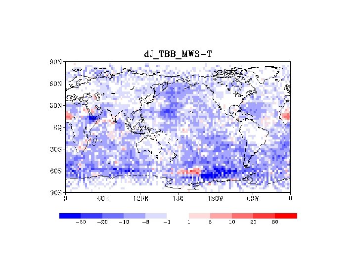
Norm dependency JMA DRY TE JMA WET TE JMA Specific humidity l Impacts of humidity sensor (MWI, AMSUB/MHS, and CSR) become clear when we use WET TE or Q norm than DRY TE norm. l Impacts of humidity non sensitive data (AMSU-A, AMV, etc) are still large in the case of WET and Q norm.

Wrong data detection l This figures shows impacts of AMSU -A/METOP 2 in two NWP systems, TEST and CNTL. p CNTL uses adequate observation error settings (operational settings). p TEST uses inadequately small observation error setting for channel eight. Solid line: CNTL Black square: TEST l The AD-based method can detect wrong observations which degenerate forecast accuracy. Relative forecast de error reduction
 QJRMS")
TL-based method 14 Ishibashi (2011) QJRMS

TL-based method K K’ Only the case that D is block diagonal. 15 Ishibashi (2011) QJRMS

TL-based estimation The formulation of TL-based observation impact estimation • Linear decomposition of analysis increments Two datasets P and Q Here, we introduced partial increment vectors (PIVs), as follows; The PIV represent a linear observation impact of each dataset. However, PIV calculation requires explicit construction of K. • Linear decomposition of departures We can calculate PIVs by using PDVs without explicit construction of K in 4 D-Var. Here, we introduced partial departure vectors (PDVs), as follows; 16
 QJRMS")
TL-based method 17 Ishibashi (2011) QJRMS

TL-based method • • • This figure shows the CNV-PIV and the TBB-PIV for Var. BC (variational bias correction) variables of the AMSU-A sensor of the NOAA 16 satellite. We can find finite contribution from the CNV. This result suggests the existence of a stability effect of the CNV for the Var. BC 18 variables (Auligné et al. , 2007) at least qualitatively.
 QJRMS")
TL-based method 19 Ishibashi (2011) QJRMS
 QJRMS")
TL-based method 20 Ishibashi (2011) QJRMS

TL-based method 21
 QJRMS")
TL-based method 22 Ishibashi (2011) QJRMS
 QJRMS")
TL-based method 23 Ishibashi (2011) QJRMS
 Tellus 24")
Formulation of AD-based method using Taylor series Errico (2007) Tellus 24
 QJRMS")
Formulation of AD-based method using PIVs 25 Ishibashi (2011) QJRMS
 QJRMS")
Cross terms 26 Ishibashi (2011) QJRMS

2. Covariance matrix optimization

Relationships between observation impact estimations and covariance optimizations • Two types of error covariance matrix optimization methods. 1. Expectation-based method p This method optimizes error covariance matrices based on theoretical relation ships; p Desroziers and Ivanov (2001), Desroziers et al (2005), and Chapnik et al (2004, 2006) 2. Sensitivity-based method p This method uses sensitivity of forecast errors respect to covariance matrices; p Daescu (2008) , Daescu and Todling (2010). • Each optimization methods include a linear observation impact estimation. 1. Expectation-based method includes DFS calculation. 2. Sensitivity-based method includes AD-based estimation. Here, Let’s see the sensitivitybased method

Sensitivity on covariance matrices

Diagnoses of the JMA global 4 D-Var l Sensitivity calculation results in August 2010. l Using dry total energy norm with 15 hr forecasts. l The results show that B is too small and R is too large in average.

Diagnoses of the JMA global 4 D-Var Radiances

Diagnoses of the JMA global 4 D-Var
 Improvement rate: Temperature hPa Pressure (1000 -")
Single case experiment Forecast time (3 days) Improvement rate: Temperature hPa Pressure (1000 - 100 h. Pa) Improvement rate: Zonal wind Results of a single case experiment of covariance optimization using the sensitivity method. l TEST uses optimized R, CNTL uses original R (operational setting). l The figure shows normalized forecast RMSE differences between TEST and CNTL: (CNTL – TEST)/CNTL. l Forecast errors decrease (increase) in warm (cold) colored regions. l Forecast error reduction by optimization is explicit.

Cycle experiment with static optimization FT 48 500 h. Pa 0 0 hPa Improvement rate FT 24 500 h. Pa Cycle days U V T Cycle days l Forecast errors increase as the cycle advances, within a week. l This may bes because of this method does not take into account cycle (nonlinear) effect, variations of background fields caused by the static optimization.
 Improvement rate: Zonal")
Cycle experiment with online optimization Pressure (1000 - 100 h. Pa) Improvement rate: Zonal wind Improvement rate: Temperature Forecast time (3 days) l One week averaged improvement rate. l To treat nonlinear effects, here, tuning coefficients are calculated each 00 UTC analysis and renewed. l Some improvement can be fond but not enough.

3. Analysis error estimation We want to know analysis errors of a DAS because of following reasons; l If we know the analysis errors, we can start researches on what parts of the DAS causes those errors toward improvement of the DAS. l We can start to design future observational systems, which can detect the analysis errors of current DASs. l Since, analysis error estimation is the same with construction of more accurate analysis than current DASs. Such analyses may be able to use as “pseudo truth”. The pseudo truth can be used validation of forecasts and operational analyses, and those of OSSEs. or directly use as in re-analyses. l Our approach is “Collect more information and integrate them correctly”

Key analysis error l The relationship between sensitivity vector and analysis error vector ( Rabier et al, 1996) C is metrics, M is TL model, a is a scalar coefficient. l Analytical determination of the coefficient a (Isaksen et al, 2005)

Key analysis error l Geometric illustration of the coefficient ‘a’ l Analysis error estimation using sensitivity vector Forecast error 1. Measure forecast error: Analysis error is too small to measure directly. 2. Propagate information using an adjoint model toward initial time Optimization: To subtract an estimated analysis error from the original analysis. is enough large to measure with enough accuracy

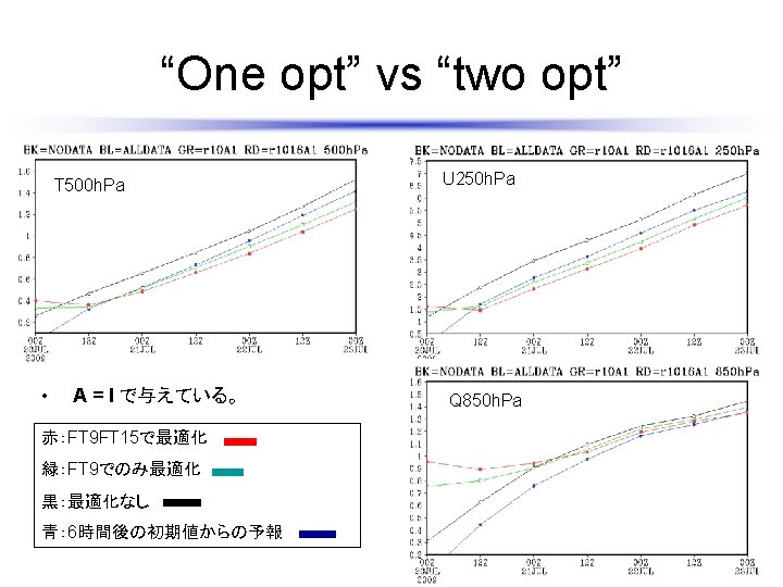
Accuracy of optimized forecast T 500 h. Pa U 250 h. Pa • Optimization time is FT 15 hr. • Vertical axis is RMSE, horizontal axis is forecast time, zero to three days. Red: optimized forecast Black: Original forecast (Blue: forecast from an original next analysis time original ) Q 850 h. Pa
 Klinker et al 1998")
Variational formulation of key analysis error Cost function Minimize J(δx) Klinker et al 1998 Here, M: TL model, δx:analysis increment vector, A: norm define matrix. Analysis increment l This method put 100% confidence on reference analysis information, since any compatible information are used. l This property causes inconsistency between observations and a background field (Klinker et al 1998, Isaksen et al 2005, Pu, Carron). l So, previous studies stop iteration at once or dozen times to avoid over fitting.

Problem of key analysis error Jo terms SOSE: Sensitivity observing system experiment (Marseille et al 2008) l Although the optimized analysis based on the key analysis error can generate more accurate forecasts, there is problems that the optimized analyses are inconsistent with observations (Isaksen et al 2005). Next, we consider to achieve analysis fields that are able to generate more accurate forecasts and consistent with observations, simultaneously.
 42")
SOSE Adapted from Marseille et al (2008 Tellus A) 42

Data assimilation theory based method l Conditional PDF Ordinary 4 D-Var l Add reference analysis fields information Extended 4 D-Var with reference analyses information X: analysis, Y: observations Xb : background field l Analytical solution has an error covariance matrix A of reference information in Kalman gain, and forecast error in input data, as follows, Xref: reference analyses

Data assimilation theory based method l We ignore cross terms. Validity of this assumption is checked by forecast errors and observation fitting. l We give A as diagonal matric, and variances of A are give as 30% of forecast error variance of background field multiplied by inflation factor f.

Accuracy of optimized forecasts 500 h. Pa Temperature 250 h. Pa Zonal wind *Inflation factor is one. • Optimized forecast with four reference analyses of every 6 hours. • Optimized forecast with only two reference analyses • Original forecast from 6 hours after initial.

Assimilation of reference analyses l The inflation factor dominates the fittings of analysis to observations. l The inflation factors larger than 500 achieve goog fitting nearly the original 4 D-Var.

Inflation and forecast accuracy l Inflation factors smaller than 500 have almost same forecast accuracy during fast 4 days, and after 5 days, larger inflation factors have smaller forecast errors, l Inflation 5000 has smaller improvement during 4 days, however, smaller errors after 5 days.

Two weeks statistics l Forecast accuracy keeps until 9 days with 95% statistical significance until 6 or 7 days.

Two weeks statistics l Forecast accuracy keeps until 9 days with 95% statistical significance until 6 or 7 days.

Fast and slow growing error modes Fast growing mode Slow growing mode plane l Key analysis error based optimized analysis increment vector exist within grey corn. Precession motions are free with in the corn. l Slow modes are constrained by observations and a background field, so constrain of these data is nearly cylinder shape. l The both achieve narrow corn constrain.

Optimized analysis increments and background error 072000 l Color shade: Optimized increments, red=plus, blue=minus. l Green contour: 500 h. Pa height. l Black contour: Integrated background error, solid lines=plus, dotted lines=minus.

Optimized analysis increments and background error 072012 l Color shade: Optimized increments, red=plus, blue=minus. l Green contour: 500 h. Pa height. l Black contour: Integrated background error, solid lines=plus, dotted lines=minus.

Optimized analysis increments and background error 072100 l Color shade: Optimized increments, red=plus, blue=minus. l Green contour: 500 h. Pa height. l Black contour: Integrated background error, solid lines=plus, dotted lines=minus.

Optimized analysis increments and background error 072112 l Color shade: Optimized increments, red=plus, blue=minus. l Green contour: 500 h. Pa height. l Black contour: Integrated background error, solid lines=plus, dotted lines=minus.

Optimized analysis increments and background error 072200 l Color shade: Optimized increments, red=plus, blue=minus. l Green contour: 500 h. Pa height. l Black contour: Integrated background error, solid lines=plus, dotted lines=minus.

Optimized analysis increments and background error 072212 l Color shade: Optimized increments, red=plus, blue=minus. l Green contour: 500 h. Pa height. l Black contour: Integrated background error, solid lines=plus, dotted lines=minus.

Optimized analysis increments and background error 072300 l Color shade: Optimized increments, red=plus, blue=minus. l Green contour: 500 h. Pa height. l Black contour: Integrated background error, solid lines=plus, dotted lines=minus.

Comparison between original analysis and optimized analysis

Optimized : FT 48 500 h. Pa T

Original: FT 48 500 h. Pa T
 Improvement rate: Height")
Pseudo truth with AD-based method Pressure (1000 - 1 h. Pa) Improvement rate: Height Forecast time (3 days) Improvement rate: Zonal wind

Maxwell demon ? We know only statistical property of data, R and B. Lets think about a system on thermal equilibrium at temperature T. We know only statistical property of the system, temperature T. While, If we can know velocity of each particle, we can get usable energy from this max entropy state, This is the Maxwell demon. We know property of each observation and can use this information.

Summary Observation impact l We defined two types of observation impact; the linear impact and the nonlinear impact. l Diagnoses of the JMA global 4 D-Var shows almost all observational dataset types contribute forecast error reduction in monthly averages. l The diagnoses imply that it is possible to derive more information from radiance data by improving usage of these data. l TL-based method is formulated. l We can see time evolutions and space distribution of each dataset impact, and evaluate them by comparison with integrated background errors. Covariance matrix optimization l Optimization methods include observation impact estimations. l Sensitivity based method diagnosed the JMA GDAS has too large (small) R (B). l The single case experiment of optimization showed the explicit forecast error reductions.
 l However, static optimization results conclude degenerate of forecast")
Summary Covariance matrix optimization (continue) l However, static optimization results conclude degenerate of forecast accuracy with cycle advances. l Online optimization also can not achieve enough improvement in this preliminary experiment. Analysis error estimation l We constructed new method based on data assimilation theory. The method assimilate reference analysis fields. l The method reduce forecast error explicitly and also consistent with observations when inflation factor is used.

Thank you very much for kind attention. Comments or Questions ? Please speak very slowly! One sentence question welcome!! More long complicated questions also welcome, but answer will be after this session or by email. I’m so sorry for my insufficient English.

BACKUPSLIDES

845 Thank you for listening Comments or Questions ? Please speak very slowly! One sentence question welcome!! Mathematical language also welcome! More long complicate questions also welcome, but answer will be after this session or by email. So sorry my very developing stage English.

Cycle experiment with static optimization FT 48 500 h. Pa 0 0 hPa Improvement rate FT 24 500 h. Pa Cycle days U V T Cycle days l Forecast errors increase as the cycle advances, within a week. l This may bes because of this method does not take into account cycle (nonlinear) effect, variations of background fields caused by the static optimization.
 Improvement rate: Zonal")
Cycle experiment with online optimization Pressure (1000 - 100 h. Pa) Improvement rate: Zonal wind Improvement rate: Temperature Forecast time (3 days) l One week averaged improvement rate. l To treat nonlinear effects, here, tuning coefficients are calculated each 00 UTC analysis and renewed. l Some improvement can be fond but not enough. Because convergence of coefficients is bad. Because large STD.

845

TL-based method Before After 72

Sensitivity on covariance matrices

2. Covariance matrix optimization STD of background err STD of departure In general, B is too large especially for humidity sensitive sensors.

2. Covariance matrix optimization STDofofbackground observationerr STD STDofofdeparture In general, R is too large especially for humidity sensitive sensors.
 Analysis increment Klinker et")
Variational formulation of key analysis error Cost function Minimize J(δx) Analysis increment Klinker et al 1998 Here, ? M: TL model, δx:analysis increment vector, A: error covariance matrix of these information We can see the sensitivity analysis is an approximate of this optimization wit only once iteration. 感度場による解析が解析解の良い近似となる条件 これを満たす場合は 2とおりある。 ① がMの特異値 1/aに属する 特異ベクトルである。 ② ①は任意の摂動が特異値-aで発展することを意味する。少 なくとも,変数変換をしない場合は物理的にありえない。
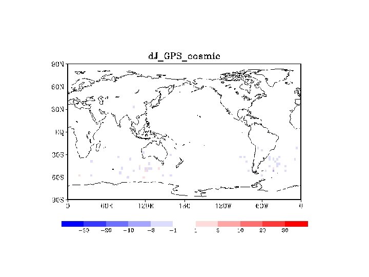
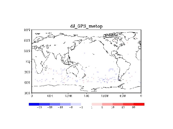
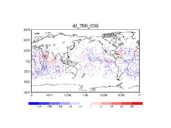
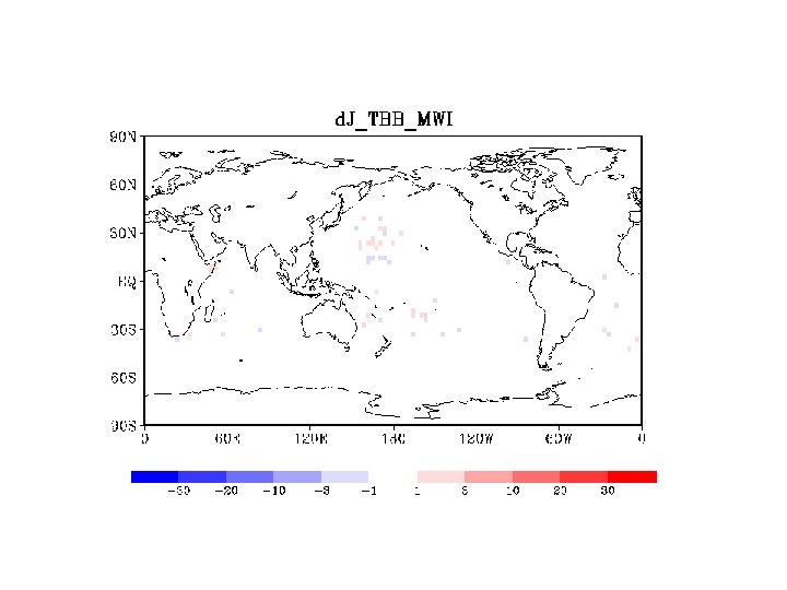

SONDE

COSMIC

Optimization with DIC • Theoretical relationships; Where, Jo and Jb are observation term, and background term of cost function, respectively • In real DASs, these relation ships are generally not satisfied because error covariance matrices using in the DASs are different from true ones. • DIC tunes B and R using in the DASs to satisfy these relation ships. 2

DIC experimental results in DAS/JMA • • About four times iteration of DIC are enough to convergence of tuning coefficients. DIC shows optimal observation error settings of satellite radiance are 20 to 30% of current settings. After DIC optimization, relation ships between value of cost function and observation data number further meet theoretical relationship; J=0. 5 N. However, we have also found OSE with these optimized covariance matrices concluded in significant forecast error increase. This is because our forecast model has large dry (wet) biases in mid (low) altitude troposphere, and DIC improve these biased in analysis fields, but model give wrong strong response (rain out watervapors in ITCZ and breal Hadley circulation)

DFS in DAS/JMA • • • Definision of DFS Radiance total < Conventional total Satellite total > others – Sattelite includes raiances, scatterometer derived winds, and satellite winds – Others=conventional – AMV-SCAT • JMA DFS Conventional total SCAT AMV aviation sonde Radiance total Largest contribution from AMSU-A/B. Ref: Result in ECMWF ( copied from Rabier 2005) DFS (%) Pilot+Temp<Amsu-A

Optimization with D 08 K
 Thermal equilibrium at temperature")
Maxwell demon ? From Bennett CH and Schumacher B (2011) Thermal equilibrium at temperature T. We can get usable energy from max entropy state with Maxwell demon. It knows velocity of each particle, while we know only statistical property, temperature. Only Statistical property, R and B. We know property of each observation and can use this information.

845 Thank you for listening Comments or Questions ? Please speak very slowly!
- Slides: 98