Estimation of Cn 2 Refractive Index Structure Constant

Estimation of Cn 2 (Refractive Index Structure Constant) in Non-Kolmogorov Deep Turbulence using Unwrapped Phase Information 18 -November-2014 Rao Gudimetla (AFRL/RDSMA) Jeremy Bos(NRC Associate) Kihei, Maui, HI 96753 Integrity Service Excellence Unclassified 1

Acknowledgement and Disclaimer This work was funded as a Laboratory Research Initiation Request by AFOSR (Air Force Office of Scientific Research) to Rao Gudimetla as principal investigator. Dr. Jeremy Bos is supported by NRC Associateship program at AFRL/Directed Energy Directorate The views expressed in this presentation are those of the authors and do not necessarily represent the views of the Department of Defense or its components. 2 Unclassified 2

Introduction 1. We present a method for estimating Cn 2 in deep turbulence using phase based information only. 2. We unwrap the phase from the complex field and use its variance and covariance to estimate the Cn 2. 3. Described approach is new and not yet published in the literature to the best of our knowledge 3 Unclassified 3

Outlines 1. Estimate the Unwrapped Phase Variance (UPV) and the corresponding Phase Correlation (UPC) 2. Estimate the Unwrapped Phase (UP) from Complex Field data 3. Estimate Cn 2 in deep turbulence 4. Conclusions 4 Unclassified 4

Example Phase Fluctuation Studies 1. Bouricius, G. M. B. , & Clifford, S. F. , J. Opt. Soc. Ame. , 60(11), 1484 -1489, (1970). 2. V. P. Lukin, “Atmospheric Adaptive Optics, “(SPIE Optical Engineering Press, Bellingham, Washington, 1995), pp. 85 -90 3. Silbaugh, Eric E. , Byron M. Welsh, and Michael C. Roggemann, " J. Opt. Soc. Ame. A 13, no. 12 (1996): 2453 -2460. 4. J. Elon Graves and Daniel L. Mc. Kenn, Proc. SPIE 1542, Active and Adaptive Optical Systems, 262 (December 1, 1991) 5. Albert D. Wheelon, “Electromagnetic Scintillation, Vol. 1 (Geometrical Optics), ” (Cambridge University Press, 2001, Cambridge). 6. L. C. Andrews and R. L. Phillips, ”Laser Beam Propagation through Random Medium, ” SPIE Press, Bellingham, Washington, 2005 5 Unclassified 5

Example Unwrapped Phase and Related Studies 1. David L. Fried and Jeffrey L. Vaughn, Appl. Opt. , Vol. 31, Issue 15, pp. 2865 -2882 (1992) 2. David L. Fried, ” J. Opt. Soc. Ame. A, Vol. 15, Issue 10, pp. 27592768 (1998) 3. Todd M. Venema and Jason D. Schmidt, ” Opt. Exp. , Vol. 16, No. 10, pp. 6985 -6998 (2008) 4. R. M. Goldstein, H. A. Zebker, and C. L. Werner, Rad. Sci. , Vol. 23, Number 4, pages 713 -720, July-August 1988, Matlab code is available from Matlab Central File Exchange 5. Dennis C. Ghiglia and Mark D. Pritt, ”Two-Dimensional Phase Unwrapping, Theory, Algorithms and Software, ” (John Wiley and Sons , New York, 1998) 6 Unclassified 6

Recent Example papers for Extraction of Atmospheric Parameters in Deep Turbulence after Phase Reconstruction 1. T. J. Brennan and D. C. Mann, Proc. SPIE, Vol. 7816 in Advanced Wavefront Control: Methods, Devices and Applications VIII, San Diego, California, August 2010. 2. V. A. Kulikov, M. S. Andreeva and V. I. Shmalhausen, Proc. SPIE, Vol. 8517 in Laser Communication and Propagation through the Atmosphere and Oceans, San Diego, California, August 2010. 3. Darryl J. Sanchez and Dennis W. Oesch, Proc. SPIE. 8520, Unconventional Imaging and Wavefront Sensing 2012 852004 (October 15, 2012) 7 Unclassified 7

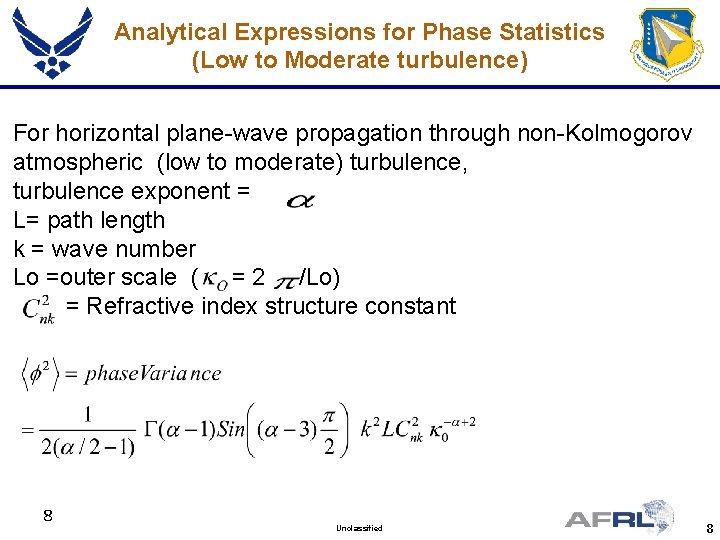
Analytical Expressions for Phase Statistics (Low to Moderate turbulence) For horizontal plane-wave propagation through non-Kolmogorov atmospheric (low to moderate) turbulence, turbulence exponent = L= path length k = wave number Lo =outer scale ( = 2 /Lo) = Refractive index structure constant 8 Unclassified 8

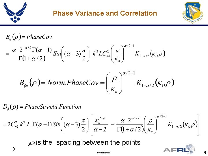
Phase Variance and Correlation 9 is the spacing between the points Unclassified 9

Approach and Key Assumptions (1) We use phase covariance data to estimate Lo (2) Then using this Lo and phase variance data, we estimate Cn 2 (3) Although phase statistics equations are derived at low turbulence levels, the unwrapped phase simulation data justifies that they are also valid in higher turbulence levels for unwrapped phase. (4) Rotational phase is not included in the phase estimation (5) Goldstein Phase Unwrapping algorithm is used 10 Unclassified 10

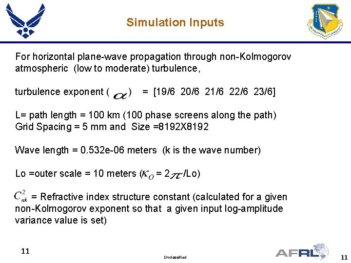
Simulation Inputs For horizontal plane-wave propagation through non-Kolmogorov atmospheric (low to moderate) turbulence, turbulence exponent ( ) = [19/6 20/6 21/6 22/6 23/6] L= path length = 100 km (100 phase screens along the path) Grid Spacing = 5 mm and Size =8192 X 8192 Wave length = 0. 532 e-06 meters (k is the wave number) Lo =outer scale = 10 meters ( =2 /Lo) = Refractive index structure constant (calculated for a given non-Kolmogorov exponent so that a given input log-amplitude variance value is set) 11 Unclassified 11

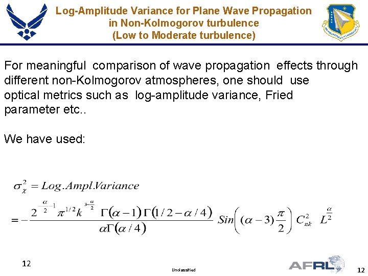
Log-Amplitude Variance for Plane Wave Propagation in Non-Kolmogorov turbulence (Low to Moderate turbulence) For meaningful comparison of wave propagation effects through different non-Kolmogorov atmospheres, one should use optical metrics such as log-amplitude variance, Fried parameter etc. . We have used: 12 Unclassified 12

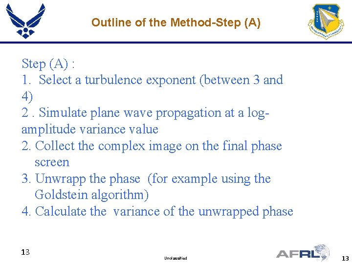
Outline of the Method-Step (A) : 1. Select a turbulence exponent (between 3 and 4) 2. Simulate plane wave propagation at a logamplitude variance value 2. Collect the complex image on the final phase screen 3. Unwrapp the phase (for example using the Goldstein algorithm) 4. Calculate the variance of the unwrapped phase 13 Unclassified 13

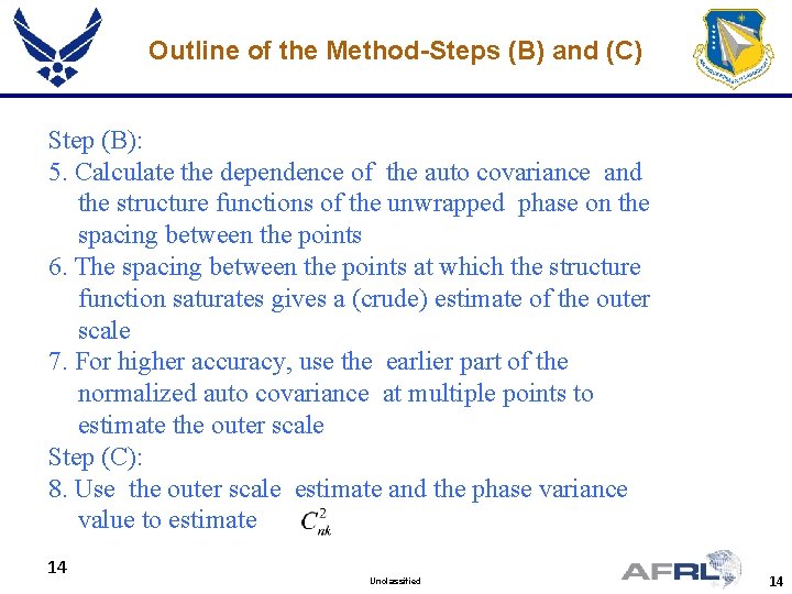
Outline of the Method-Steps (B) and (C) Step (B): 5. Calculate the dependence of the auto covariance and the structure functions of the unwrapped phase on the spacing between the points 6. The spacing between the points at which the structure function saturates gives a (crude) estimate of the outer scale 7. For higher accuracy, use the earlier part of the normalized auto covariance at multiple points to estimate the outer scale Step (C): 8. Use the outer scale estimate and the phase variance value to estimate 14 Unclassified 14

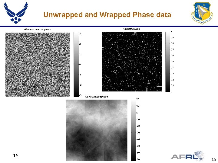
Unwrapped and Wrapped Phase data 15 Unclassified 15

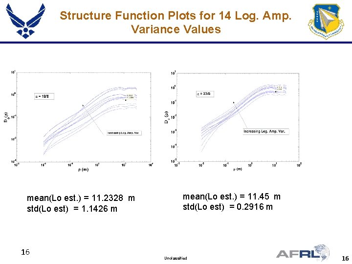
Structure Function Plots for 14 Log. Amp. Variance Values mean(Lo est. ) = 11. 2328 m std(Lo est) = 1. 1426 m 16 mean(Lo est. ) = 11. 45 m std(Lo est) = 0. 2916 m Unclassified 16

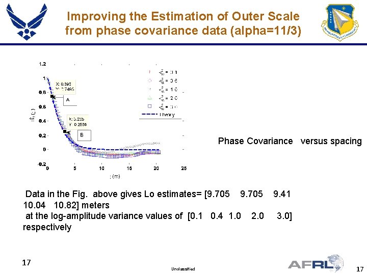
Improving the Estimation of Outer Scale from phase covariance data (alpha=11/3) Phase Covariance versus spacing Data in the Fig. above gives Lo estimates= [9. 705 9. 41 10. 04 10. 82] meters at the log-amplitude variance values of [0. 1 0. 4 1. 0 2. 0 3. 0] respectively 17 Unclassified 17

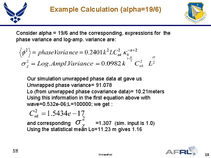
Example Calculation (alpha=19/6) Consider alpha = 19/6 and the corresponding, expressions for the phase variance and log-amp. variance are: Our simulation unwrapped phase data at gave us Unwrapped phase variance= 91. 078 Lo (from unwrapped phase covariance data)= 10. 21 meters Using this information in the first equation above with wave=0. 532 e-06; L=100000; we get : and corresponding =1. 307 (sim. input is 1. 0) Using the statistical mean Lo=11. 23 m gives 1. 16 18 Unclassified 18

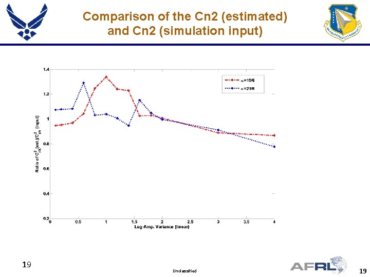
Comparison of the Cn 2 (estimated) and Cn 2 (simulation input) 19 Unclassified 19

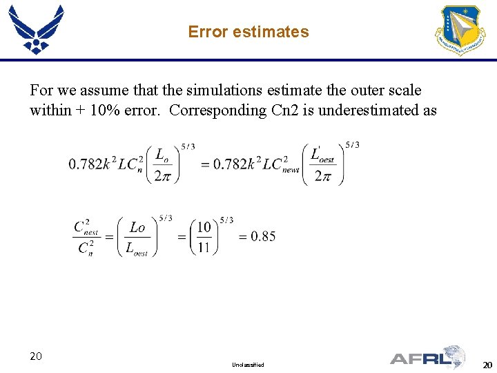
Error estimates For we assume that the simulations estimate the outer scale within + 10% error. Corresponding Cn 2 is underestimated as 20 Unclassified 20

Conclusions 1. A new Cn 2 extraction completely based on phase information is described 2. Extraction needs phase from large arrays depending on the outer scale value 3. Additional studies are needed to examine the stability of the extraction procedure in the presence of noise 21 Unclassified 21

22 Unclassified 22

Unclassified 23