Estimation Econometra ADE Estimation We assume we have

Estimation Econometría. ADE.

Estimation • We assume we have a sample of size T of: – The dependent variable (y) – The explanatory variables (x 1, x 2, x 3, …, xk), with x 1 being an intercept (a column vector of 1 s) • We also have a vector of unknown parameters b=(b 1, b 2, …, bk)’ • We have a perturbation vector (u) of dimension T • A set of hypothesis about the relationship between X, b and u.

Estimation In these circumstances, we can link the dependent and the explanatory variables as follows: Yt = b 1 + b 2 x 2 t + … + bk xkt + ut Matrix form: Y = Xb + u Compact form: Yt = xt’ b + ut Our key problem is to provide value to the components of the vector b

Estimation To assign values to the parameters, we have some options. -We can invent them. -We can phone Rappel and ask him for the more appropriate values according to his “view”. - We can use a random procedure. - We can estimate them.

Estimation theory is a branch of statistics that deals with providing values to a set of parameters based on measured/empirical data that has a random component. An estimator attempts to approximate the unknown parameters using the measurements.

Estimation methods • Maximum likelihood • Ordinary Least Squares • Non-linear methods • GMM Which one will we use along the course?

Estimation • Do you know this John Ford’s film? • There is a very famous scene where cowboys escape from redskins by crossing the Rio Grande river. (28: 05) • Do they use a least squares principle?

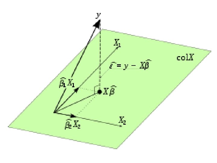
Estimation We have the following the relationship: Y=Xb+u Thus, we can express it as follows:

Estimation The OLS estimator

Estimation • • • Then, The projection matrix is: PX = X(X’X)-1 X’ The residual matrix is: M = I - PX = I - X(X’X)-1 X’ PX and M are orthogonal PX is symmetric (PX= P’X ) PX is idempotent (PX PX= PX )

Estimation • Consequently, we have that:

Estimation • By simply comparing the equation, we obtain the expression of the ordinary least squares (OLS) estimator:

Estimation We can alternatively obtain this same result by simply applying the least squares principle: • We need to get the combination of values of the estimation vector that minimizes the sum of the squared residuals. • Analytically, this implies to solve this:

Estimation

Properties of the LS Estimator We have obtained the LS estimator. But, is good enough this estimator? Properties - Unbiased - BLUE - Consistent - Efficient

Properties of the LS Estimator It is advisable to express the LS estimator as follows:

Properties of the LS Estimator Thus, we have that: The OLS estimator vector is unbiased

Properties of the LS Estimator The variance of the estimator vector is

Properties of the LS Estimator The OLS estimator is BLUE • Best Linear Unbiased Estimator • This implies that it has the lowest variance, as compared to other unbiased, linear estimators. • Gauss-Markov theorem helps us to prove it.

Properties of the LS Estimator The LS estimator is consistent if we can prove that: Or equivalently

Properties of the LS Estimator The use of plim’s can help us to prove consistency, given that:

Properties of the LS Estimator We can employ an alternative method to prove consistency. An estimator is consistent if: • It is asymptotically unbiased • Its variance goes to zero when the sample grows to infinity.

Properties of the LS Estimator The first condition is held by simply considering that:

Properties of the LS Estimator The secondition also holds.

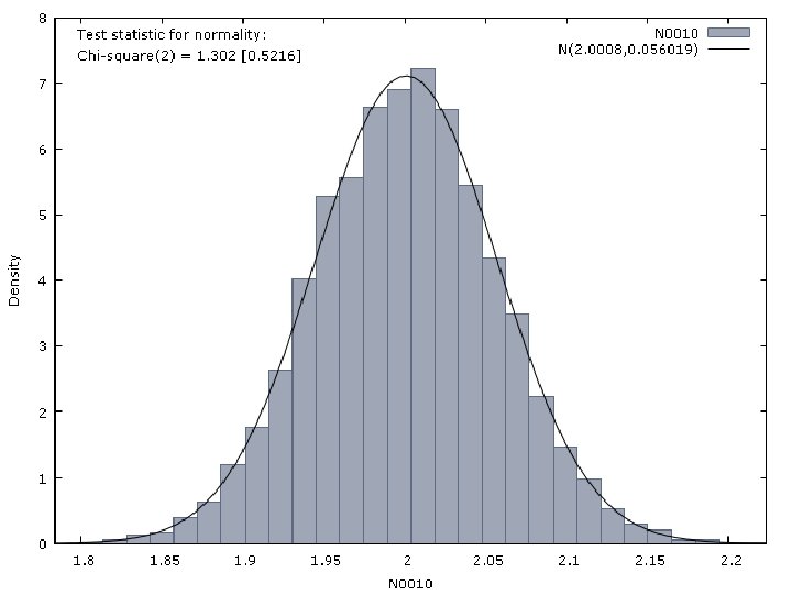
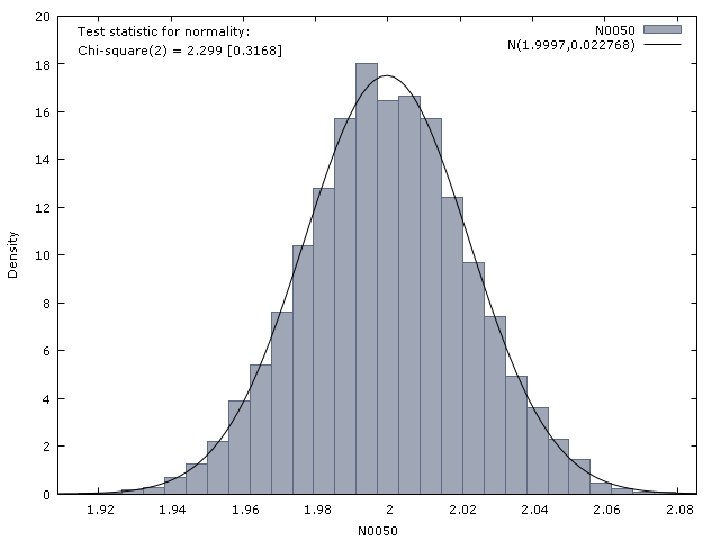
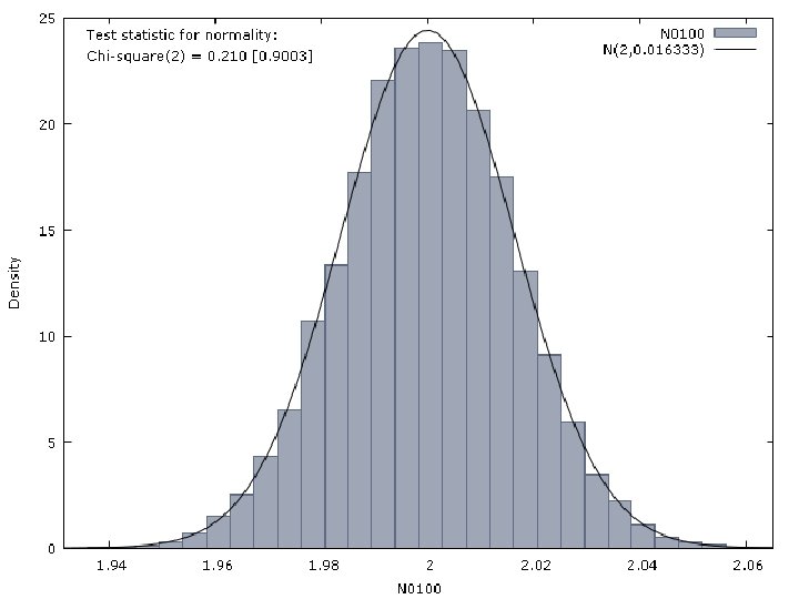
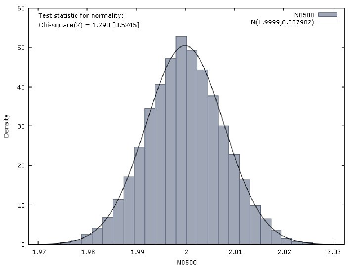
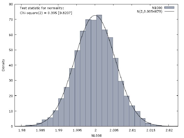
Properties of the LS Estimator We can also follow a very intuitive approach. If an estimator is consistent, we have that: • The estimator asymptotically collapses towards a value, which is the true value of the parameter. Thus, the differences between estimator and true value of the parameter vanishes. • It is also true that the higher the sample size, the more information available to estimate the model.

Properties of the LS Estimator Let us consider that the observations of a dependent variable are generated by the following model: T={10, 50, 100, 500, 1000} The perturbation is generated by a N(0, 1) distribution

Properties of the LS Estimator Then, we estimate by OLS the following model The results we have obtained are reported in next Figures.

Properties of the OLS estimator. Efficiency An estimator is efficient if it has the lowest variance, compare to other unbiased estimators.

Properties of the OLS estimator. Efficiency To prove it: • We should impose that the perturbation follows a normal distribution • We should then obtain the Cramer-Rao bound.

Properties of the OLS estimator. Efficiency • We should compare the Cramer-Rao bound with the variance of the OLS estimator. • For the OLS estimator vector, the Cramer-Rao bound is s 2 (X’X)-1. • It coincides with the covariance matrix of the OLS estimator vector. • Consequently, the OLS estimator is efficient.

OLS estimator of the variance of the perturbation. • If we assume that the perturbation vector follows a N(0, s 2 I) distribution, we have that the vector y follows a N(Xb, s 2 I) distribution. • We already know how the vector b can be estimated • We need now to get an estimator of the variance of the perturbation (s 2) • We can use the OLS approach

OLS estimator of the variance of the perturbation. The OLS estimator can be defined as follows: With being the sum of the squared residuals (SSR)

OLS estimator of the variance of the perturbation. This estimator shows the following properties: • • It is unbiased It is NOT linear It is consistent It is NOT efficient

Maximum Likelihood estimator The ML estimation selects the set of values of the model parameters that maximizes the likelihood function. • Assuming all the previous hypothesis, the joint density function of (y 1, y 2, …, y. T) can be expressed as follows:

Maximum Likelihood estimator Then, the likelihood function can be stated as follows: Which is the difference with respect the joint density function?

Maximum Likelihood estimator To obtain the ML estimators, we should first the loglikelihood function Then, we should obtain the values of the parameters that maximize this function

Maximum Likelihood estimator The solutions to this optimization problem are: The ML estimator and the OLS estimator coincide. Both have the same properties.

Maximum Likelihood estimator The ML estimator of the variance of the perturbation is: It is consistent It is not unbiased, linear, efficient It has asymptotical good properties (it is a MLE)