Estimation and Hypothesis Testing for Two Population Parameters

Estimation and Hypothesis Testing for Two Population Parameters

Chapter Goals After completing this chapter, you should be able to: n Test hypotheses or form interval estimates for n two independent population means n n Standard deviations known Standard deviations unknown two means from paired samples the difference between two population proportions

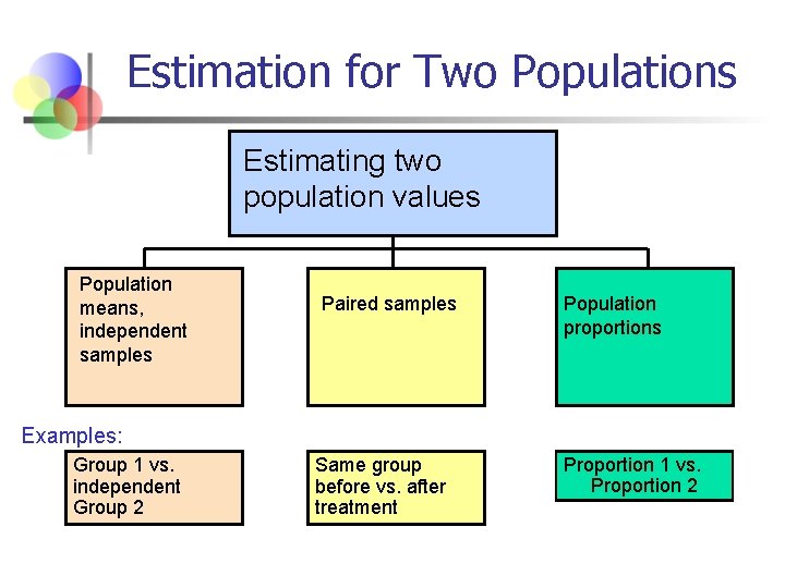
Estimation for Two Populations Estimating two population values Population means, independent samples Paired samples Population proportions Examples: Group 1 vs. independent Group 2 Same group before vs. after treatment Proportion 1 vs. Proportion 2

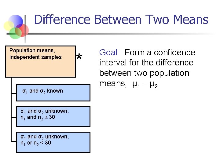
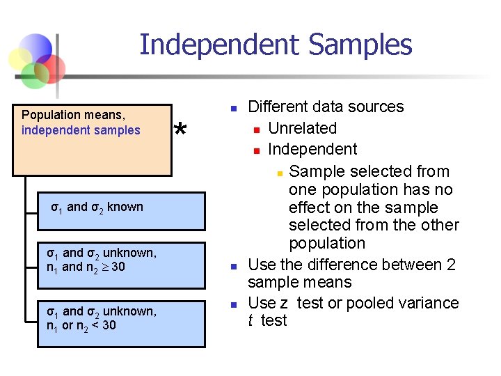
Difference Between Two Means Population means, independent samples σ1 and σ2 known σ1 and σ2 unknown, n 1 and n 2 30 σ1 and σ2 unknown, n 1 or n 2 < 30 * Goal: Form a confidence interval for the difference between two population means, μ 1 – μ 2

Independent Samples Population means, independent samples * n σ1 and σ2 known σ1 and σ2 unknown, n 1 and n 2 30 σ1 and σ2 unknown, n 1 or n 2 < 30 n n Different data sources n Unrelated n Independent n Sample selected from one population has no effect on the sample selected from the other population Use the difference between 2 sample means Use z test or pooled variance t test

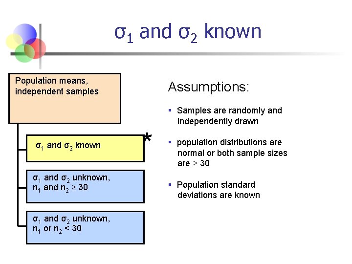
σ1 and σ2 known Population means, independent samples Assumptions: § Samples are randomly and independently drawn σ1 and σ2 known σ1 and σ2 unknown, n 1 and n 2 30 σ1 and σ2 unknown, n 1 or n 2 < 30 * § population distributions are normal or both sample sizes are 30 § Population standard deviations are known

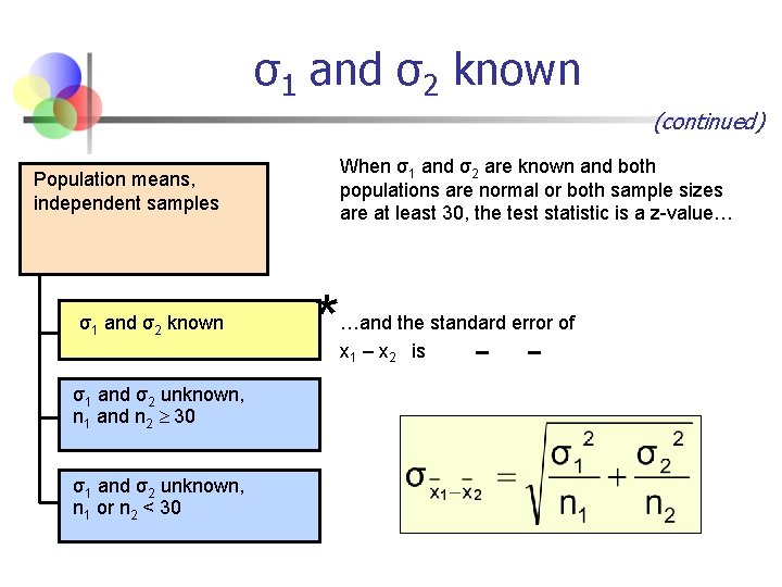
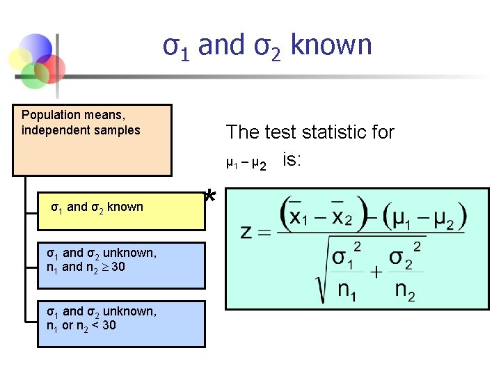
σ1 and σ2 known (continued) When σ1 and σ2 are known and both populations are normal or both sample sizes are at least 30, the test statistic is a z-value… Population means, independent samples σ1 and σ2 known σ1 and σ2 unknown, n 1 and n 2 30 σ1 and σ2 unknown, n 1 or n 2 < 30 * …and the standard error of x 1 – x 2 is

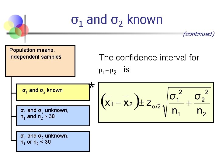
σ1 and σ2 known (continued) Population means, independent samples σ1 and σ2 known σ1 and σ2 unknown, n 1 and n 2 30 σ1 and σ2 unknown, n 1 or n 2 < 30 The confidence interval for μ 1 – μ 2 is: *

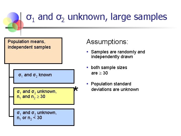
σ1 and σ2 unknown, large samples Assumptions: Population means, independent samples § Samples are randomly and independently drawn § both sample sizes are 30 σ1 and σ2 known σ1 and σ2 unknown, n 1 and n 2 30 σ1 and σ2 unknown, n 1 or n 2 < 30 * § Population standard deviations are unknown

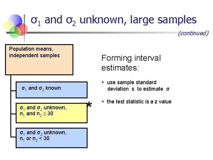
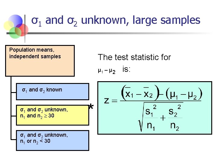
σ1 and σ2 unknown, large samples (continued) Population means, independent samples Forming interval estimates: § use sample standard deviation s to estimate σ σ1 and σ2 known σ1 and σ2 unknown, n 1 and n 2 30 σ1 and σ2 unknown, n 1 or n 2 < 30 * § the test statistic is a z value

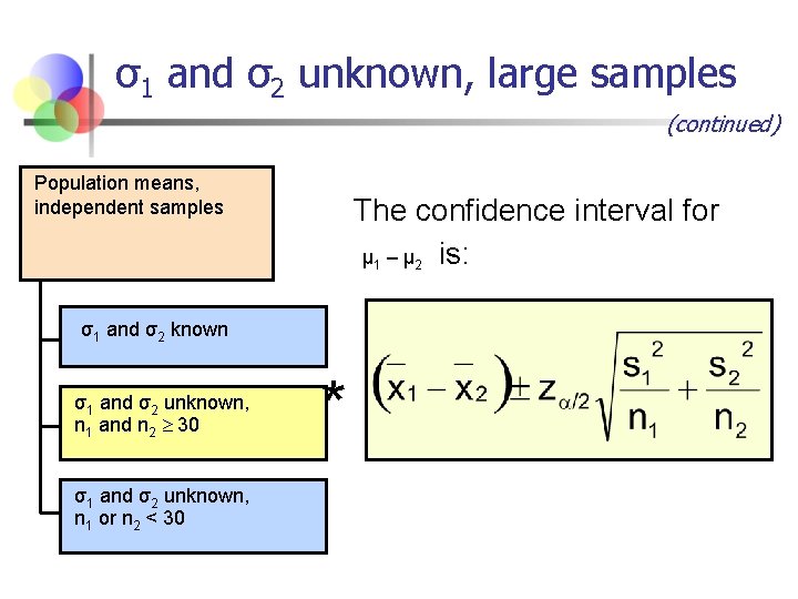
σ1 and σ2 unknown, large samples (continued) Population means, independent samples The confidence interval for μ 1 – μ 2 is: σ1 and σ2 known σ1 and σ2 unknown, n 1 and n 2 30 σ1 and σ2 unknown, n 1 or n 2 < 30 *

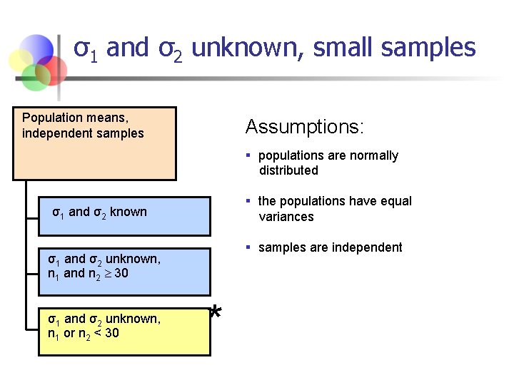
σ1 and σ2 unknown, small samples Population means, independent samples Assumptions: § populations are normally distributed § the populations have equal variances σ1 and σ2 known § samples are independent σ1 and σ2 unknown, n 1 and n 2 30 σ1 and σ2 unknown, n 1 or n 2 < 30 *

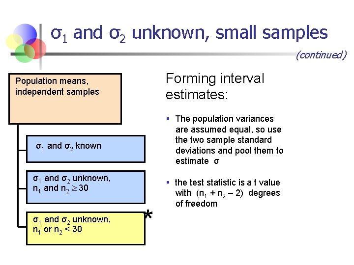
σ1 and σ2 unknown, small samples (continued) Forming interval estimates: Population means, independent samples § The population variances are assumed equal, so use the two sample standard deviations and pool them to estimate σ σ1 and σ2 known σ1 and σ2 unknown, n 1 and n 2 30 σ1 and σ2 unknown, n 1 or n 2 < 30 * § the test statistic is a t value with (n 1 + n 2 – 2) degrees of freedom

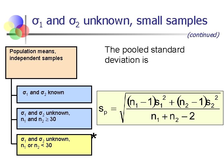
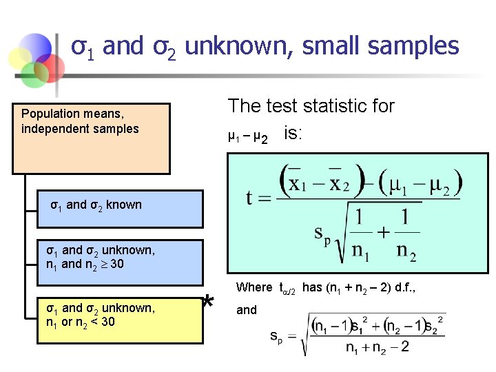
σ1 and σ2 unknown, small samples (continued) The pooled standard deviation is Population means, independent samples σ1 and σ2 known σ1 and σ2 unknown, n 1 and n 2 30 σ1 and σ2 unknown, n 1 or n 2 < 30 *

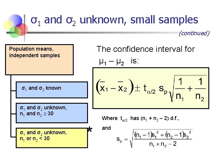
σ1 and σ2 unknown, small samples (continued) The confidence interval for μ 1 – μ 2 is: Population means, independent samples σ1 and σ2 known σ1 and σ2 unknown, n 1 and n 2 30 σ1 and σ2 unknown, n 1 or n 2 < 30 Where t /2 has (n 1 + n 2 – 2) d. f. , * and

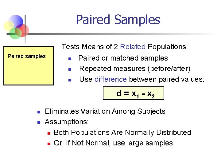
Paired Samples Tests Means of 2 Related Populations Paired samples n n n Paired or matched samples Repeated measures (before/after) Use difference between paired values: d = x 1 - x 2 n n Eliminates Variation Among Subjects Assumptions: n Both Populations Are Normally Distributed n Or, if Not Normal, use large samples

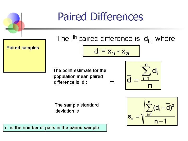
Paired Differences The ith paired difference is di , where Paired samples di = x 1 i - x 2 i The point estimate for the population mean paired difference is d : The sample standard deviation is the number of pairs in the paired sample

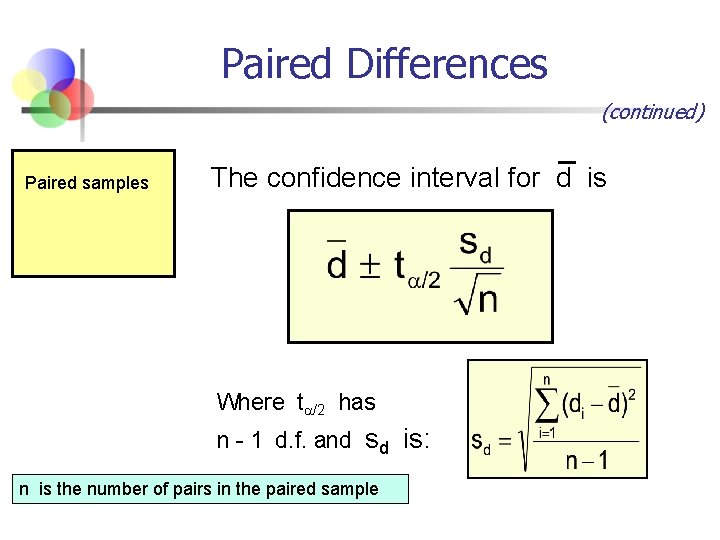
Paired Differences (continued) Paired samples The confidence interval for d is Where t /2 has n - 1 d. f. and sd is: n is the number of pairs in the paired sample

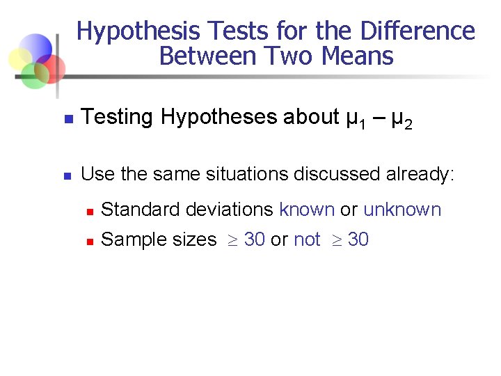
Hypothesis Tests for the Difference Between Two Means n Testing Hypotheses about μ 1 – μ 2 n Use the same situations discussed already: n Standard deviations known or unknown n Sample sizes 30 or not 30

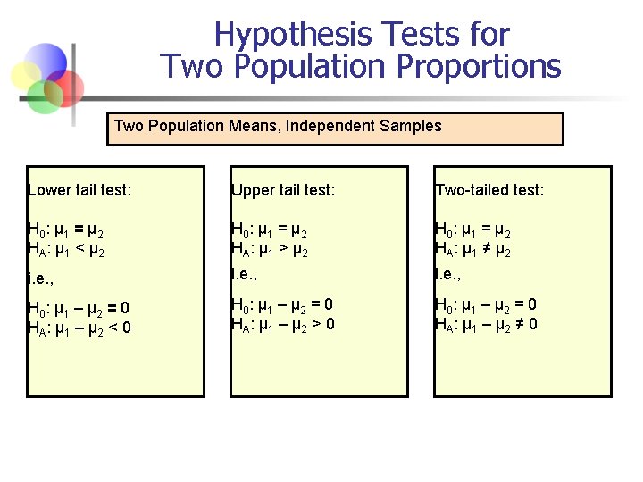
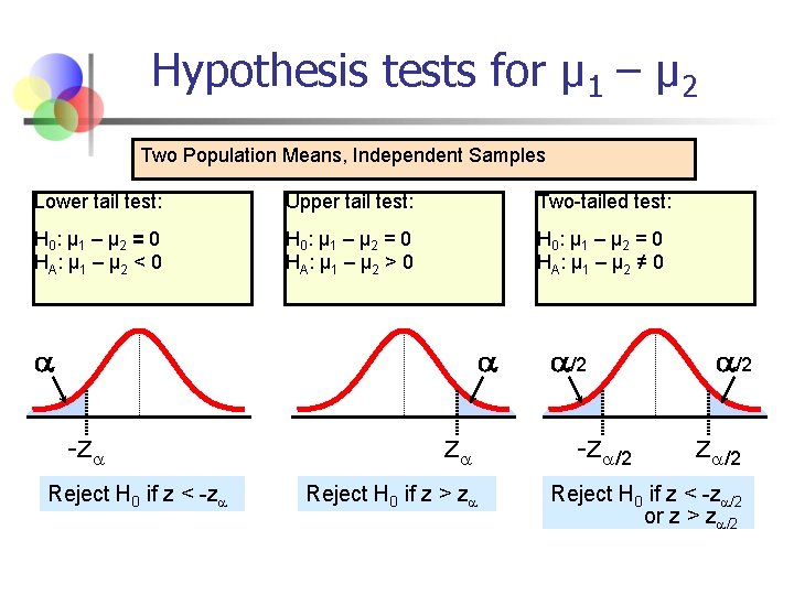
Hypothesis Tests for Two Population Proportions Two Population Means, Independent Samples Lower tail test: Upper tail test: Two-tailed test: H 0 : μ 1 = μ 2 HA: μ 1 < μ 2 H 0 : μ 1 = μ 2 HA: μ 1 > μ 2 H 0 : μ 1 = μ 2 HA: μ 1 ≠ μ 2 i. e. , H 0 : μ 1 – μ 2 = 0 HA: μ 1 – μ 2 < 0 H 0 : μ 1 – μ 2 = 0 HA: μ 1 – μ 2 > 0 H 0 : μ 1 – μ 2 = 0 HA: μ 1 – μ 2 ≠ 0

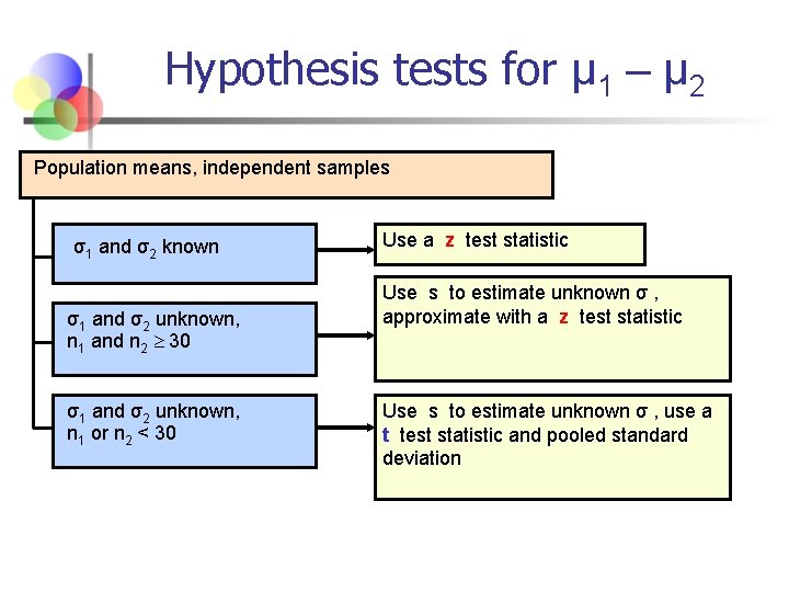
Hypothesis tests for μ 1 – μ 2 Population means, independent samples σ1 and σ2 known σ1 and σ2 unknown, n 1 and n 2 30 σ1 and σ2 unknown, n 1 or n 2 < 30 Use a z test statistic Use s to estimate unknown σ , approximate with a z test statistic Use s to estimate unknown σ , use a t test statistic and pooled standard deviation

σ1 and σ2 known Population means, independent samples σ1 and σ2 known σ1 and σ2 unknown, n 1 and n 2 30 σ1 and σ2 unknown, n 1 or n 2 < 30 The test statistic for μ 1 – μ 2 is: *

σ1 and σ2 unknown, large samples Population means, independent samples The test statistic for μ 1 – μ 2 is: σ1 and σ2 known σ1 and σ2 unknown, n 1 and n 2 30 σ1 and σ2 unknown, n 1 or n 2 < 30 *

σ1 and σ2 unknown, small samples The test statistic for μ 1 – μ 2 is: Population means, independent samples σ1 and σ2 known σ1 and σ2 unknown, n 1 and n 2 30 σ1 and σ2 unknown, n 1 or n 2 < 30 * Where t /2 has (n 1 + n 2 – 2) d. f. , and

Hypothesis tests for μ 1 – μ 2 Two Population Means, Independent Samples Lower tail test: Upper tail test: Two-tailed test: H 0 : μ 1 – μ 2 = 0 HA: μ 1 – μ 2 < 0 H 0 : μ 1 – μ 2 = 0 HA: μ 1 – μ 2 > 0 H 0 : μ 1 – μ 2 = 0 HA: μ 1 – μ 2 ≠ 0 -z Reject H 0 if z < -z z Reject H 0 if z > z /2 -z /2 Reject H 0 if z < -z /2 or z > z /2

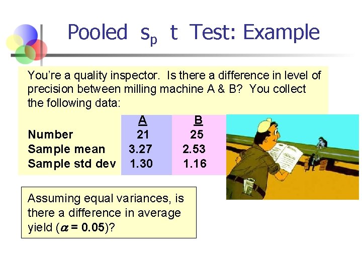
Pooled sp t Test: Example You’re a quality inspector. Is there a difference in level of precision between milling machine A & B? You collect the following data: A B Number 21 25 Sample mean 3. 27 2. 53 Sample std dev 1. 30 1. 16 Assuming equal variances, is there a difference in average yield ( = 0. 05)?

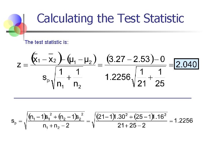
Calculating the Test Statistic The test statistic is:

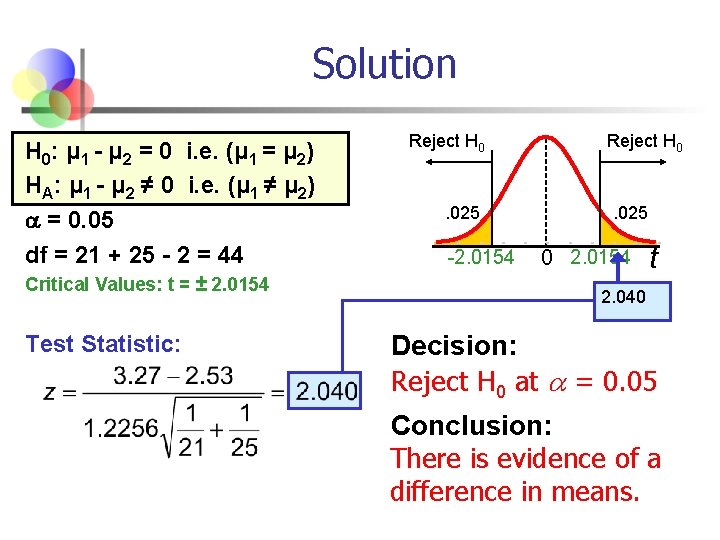
Solution H 0: μ 1 - μ 2 = 0 i. e. (μ 1 = μ 2) HA: μ 1 - μ 2 ≠ 0 i. e. (μ 1 ≠ μ 2) = 0. 05 df = 21 + 25 - 2 = 44 Critical Values: t = ± 2. 0154 Test Statistic: Reject H 0 . 025 -2. 0154 Reject H 0 . 025 0 2. 0154 t 2. 040 Decision: Reject H 0 at = 0. 05 Conclusion: There is evidence of a difference in means.

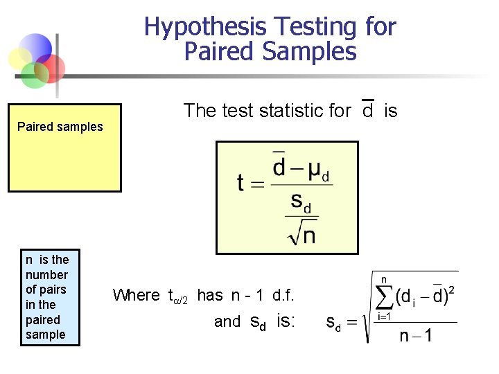
Hypothesis Testing for Paired Samples Paired samples n is the number of pairs in the paired sample The test statistic for d is Where t /2 has n - 1 d. f. and sd is:

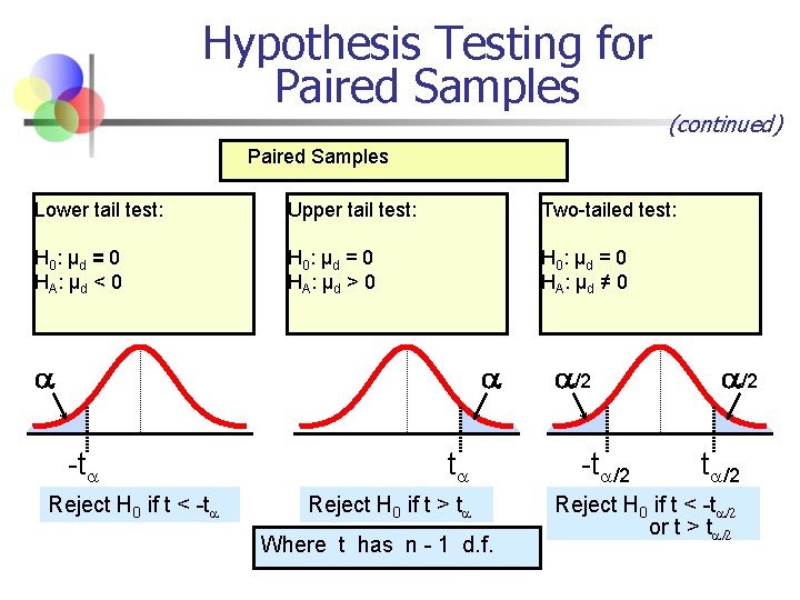
Hypothesis Testing for Paired Samples (continued) Paired Samples Lower tail test: Upper tail test: Two-tailed test: H 0 : μd = 0 HA: μd < 0 H 0 : μd = 0 HA: μd > 0 H 0 : μd = 0 HA: μd ≠ 0 -t Reject H 0 if t < -t t Reject H 0 if t > t Where t has n - 1 d. f. /2 -t /2 Reject H 0 if t < -t /2 or t > t /2

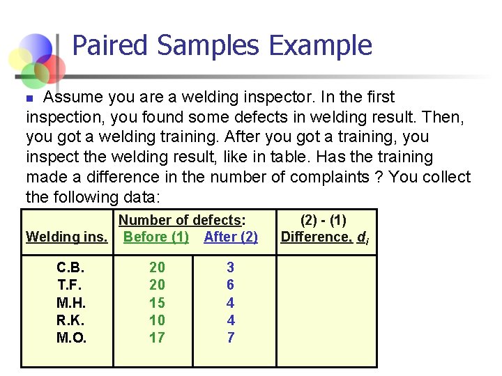
Paired Samples Example Assume you are a welding inspector. In the first inspection, you found some defects in welding result. Then, you got a welding training. After you got a training, you inspect the welding result, like in table. Has the training made a difference in the number of complaints ? You collect the following data: n Number of defects: Welding ins. Before (1) After (2) C. B. T. F. M. H. R. K. M. O. 20 20 15 10 17 3 6 4 4 7 (2) - (1) Difference, di

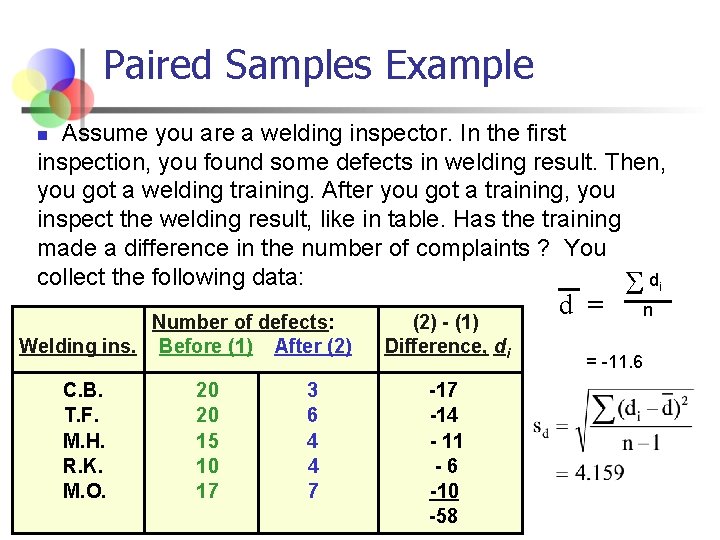
Paired Samples Example Assume you are a welding inspector. In the first inspection, you found some defects in welding result. Then, you got a welding training. After you got a training, you inspect the welding result, like in table. Has the training made a difference in the number of complaints ? You collect the following data: di n Number of defects: Welding ins. Before (1) After (2) C. B. T. F. M. H. R. K. M. O. 20 20 15 10 17 3 6 4 4 7 (2) - (1) Difference, di -17 -14 - 11 -6 -10 -58 d = = -11. 6 n

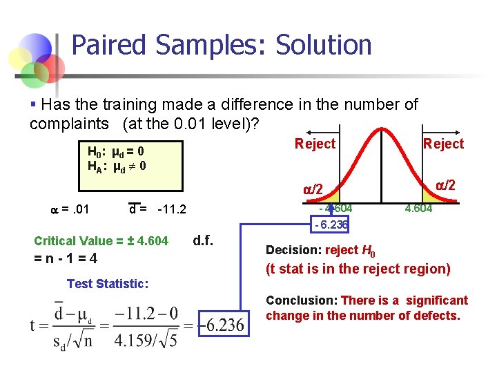
Paired Samples: Solution § Has the training made a difference in the number of complaints (at the 0. 01 level)? H 0 : μ d = 0 HA: μd 0 =. 01 =n-1=4 Reject /2 - 4. 604 - 6. 236 d = -11. 2 Critical Value = ± 4. 604 Reject d. f. 4. 604 Decision: reject H 0 (t stat is in the reject region) Test Statistic: Conclusion: There is a significant change in the number of defects.

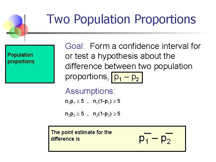
Two Population Proportions Population proportions Goal: Form a confidence interval for or test a hypothesis about the difference between two population proportions, p 1 – p 2 Assumptions: n 1 p 1 5 , n 1(1 -p 1) 5 n 2 p 2 5 , n 2(1 -p 2) 5 The point estimate for the difference is p 1 – p 2

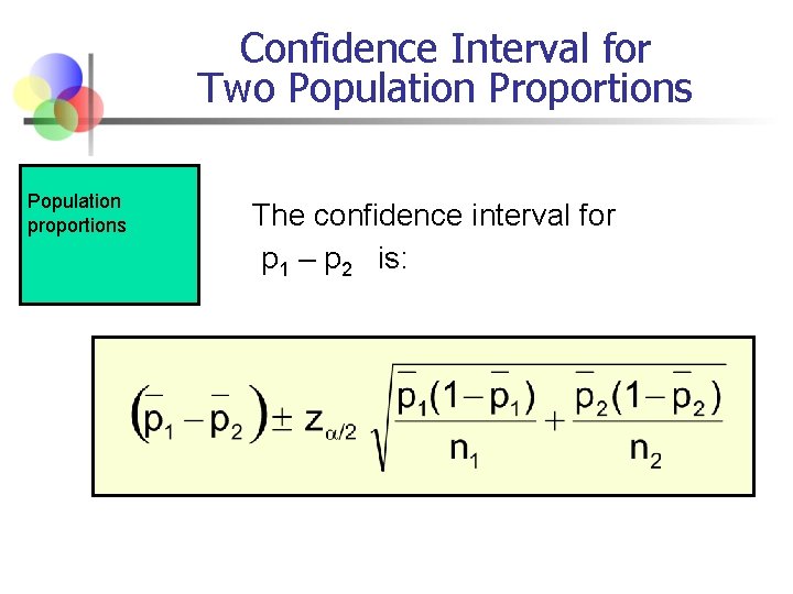
Confidence Interval for Two Population Proportions Population proportions The confidence interval for p 1 – p 2 is:

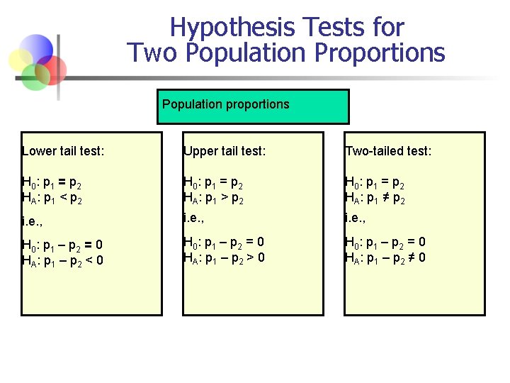
Hypothesis Tests for Two Population Proportions Population proportions Lower tail test: Upper tail test: Two-tailed test: H 0 : p 1 = p 2 HA: p 1 < p 2 H 0 : p 1 = p 2 HA: p 1 > p 2 H 0 : p 1 = p 2 HA: p 1 ≠ p 2 i. e. , H 0 : p 1 – p 2 = 0 HA: p 1 – p 2 < 0 H 0 : p 1 – p 2 = 0 HA: p 1 – p 2 > 0 H 0 : p 1 – p 2 = 0 HA: p 1 – p 2 ≠ 0

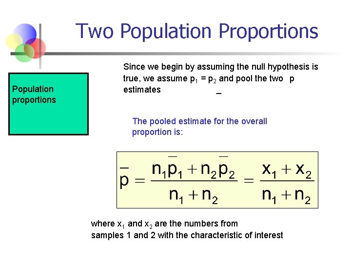
Two Population Proportions Population proportions Since we begin by assuming the null hypothesis is true, we assume p 1 = p 2 and pool the two p estimates The pooled estimate for the overall proportion is: where x 1 and x 2 are the numbers from samples 1 and 2 with the characteristic of interest

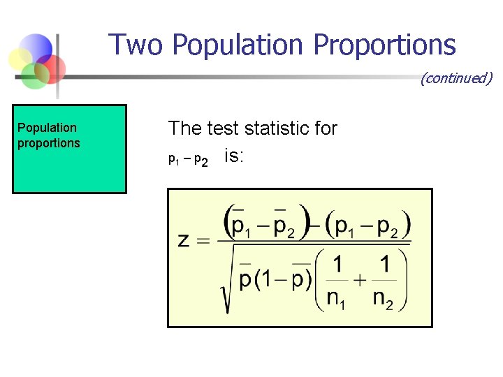
Two Population Proportions (continued) Population proportions The test statistic for p 1 – p 2 is:

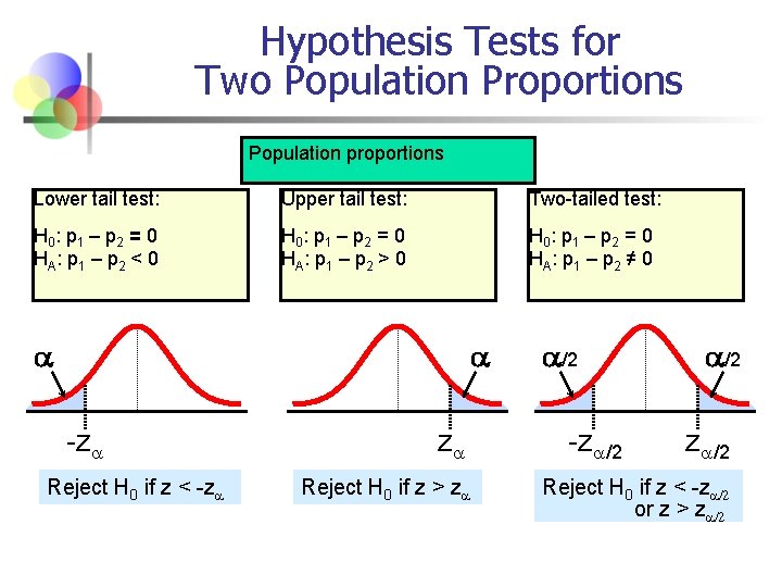
Hypothesis Tests for Two Population Proportions Population proportions Lower tail test: Upper tail test: Two-tailed test: H 0 : p 1 – p 2 = 0 HA: p 1 – p 2 < 0 H 0 : p 1 – p 2 = 0 HA: p 1 – p 2 > 0 H 0 : p 1 – p 2 = 0 HA: p 1 – p 2 ≠ 0 -z Reject H 0 if z < -z z Reject H 0 if z > z /2 -z /2 Reject H 0 if z < -z /2 or z > z /2

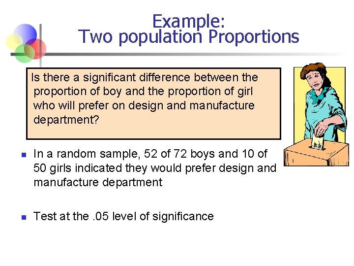
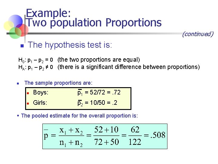
Example: Two population Proportions Is there a significant difference between the proportion of boy and the proportion of girl who will prefer on design and manufacture department? n n In a random sample, 52 of 72 boys and 10 of 50 girls indicated they would prefer design and manufacture department Test at the. 05 level of significance

Example: Two population Proportions (continued) n The hypothesis test is: H 0: p 1 – p 2 = 0 (the two proportions are equal) HA: p 1 – p 2 ≠ 0 (there is a significant difference between proportions) n The sample proportions are: n Boys: p 1 = 52/72 =. 72 n Girls: p 2 = 10/50 =. 2 § The pooled estimate for the overall proportion is:

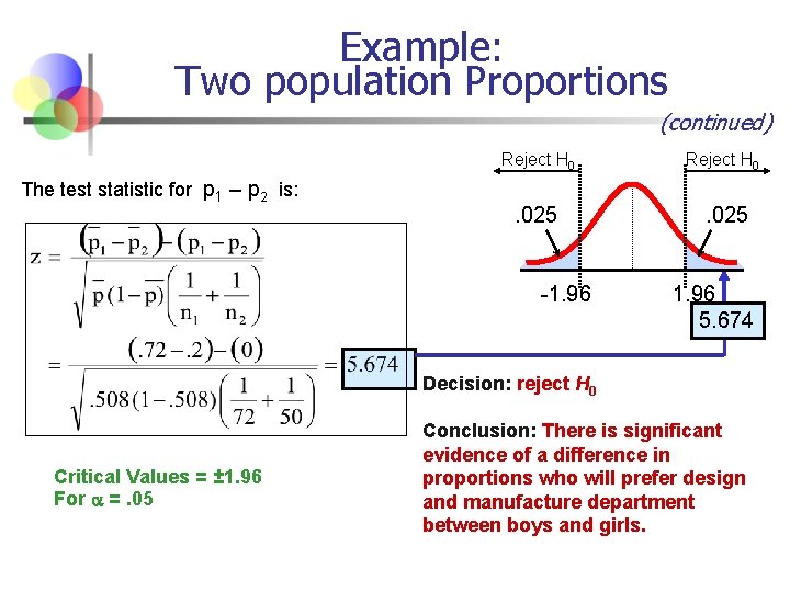
Example: Two population Proportions (continued) The test statistic for p 1 – p 2 is: Reject H 0 . 025 -1. 96 5. 674 Decision: reject H 0 Critical Values = ± 1. 96 For =. 05 Conclusion: There is significant evidence of a difference in proportions who will prefer design and manufacture department between boys and girls.

Hypothesis Tests for One and Two Population Variances Course 3

Chapter Goals After completing this chapter, you should be able to: n n Formulate and complete hypothesis tests for a single population variance Find critical chi-square distribution values from the chisquare table Formulate and complete hypothesis tests for the difference between two population variances Use the F table to find critical F values

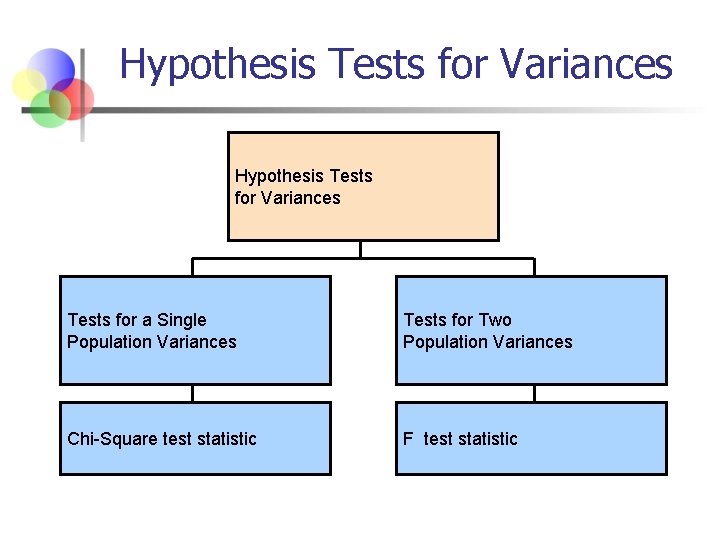
Hypothesis Tests for Variances Tests for a Single Population Variances Tests for Two Population Variances Chi-Square test statistic F test statistic

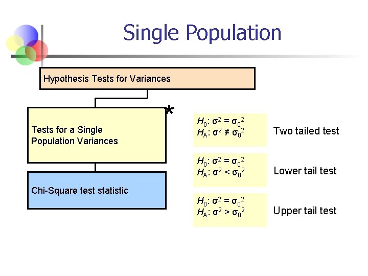
Single Population Hypothesis Tests for Variances Tests for a Single Population Variances * H 0 : σ2 = σ0 2 HA: σ2 ≠ σ02 Two tailed test H 0 : σ2 = σ0 2 HA: σ2 < σ02 Lower tail test H 0 : σ2 = σ0 2 HA: σ2 > σ02 Upper tail test Chi-Square test statistic

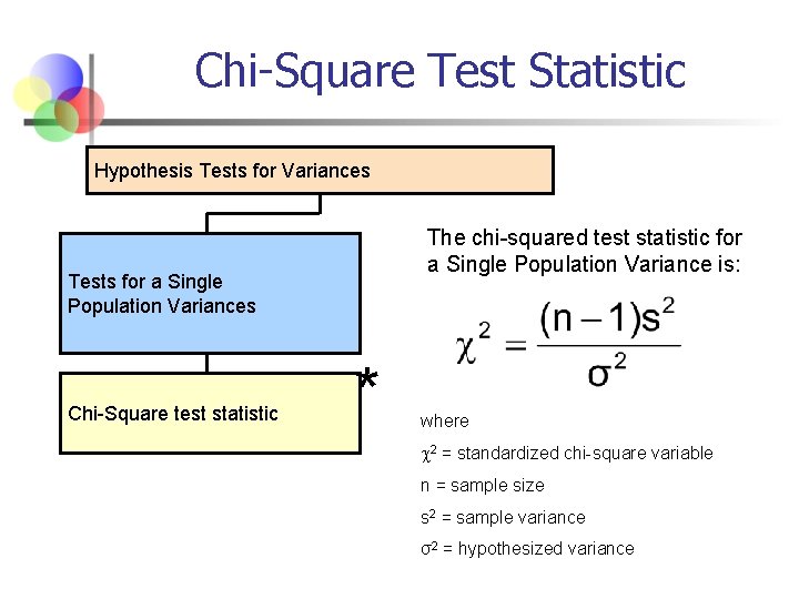
Chi-Square Test Statistic Hypothesis Tests for Variances The chi-squared test statistic for a Single Population Variance is: Tests for a Single Population Variances Chi-Square test statistic * where 2 = standardized chi-square variable n = sample size s 2 = sample variance σ2 = hypothesized variance

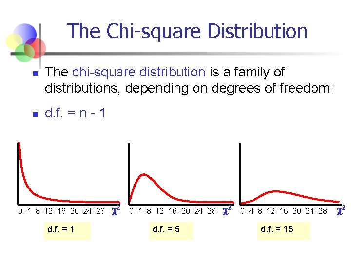
The Chi-square Distribution n n The chi-square distribution is a family of distributions, depending on degrees of freedom: d. f. = n - 1 0 4 8 12 16 20 24 28 d. f. = 1 2 0 4 8 12 16 20 24 28 d. f. = 5 2 0 4 8 12 16 20 24 28 d. f. = 15 2

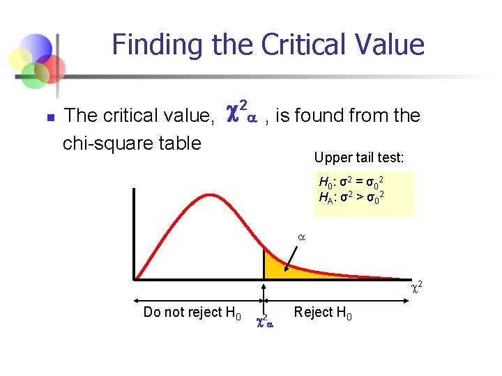
Finding the Critical Value n 2 The critical value, , is found from the chi-square table Upper tail test: H 0 : σ2 = σ0 2 HA: σ2 > σ02 2 Do not reject H 0 2 Reject H 0

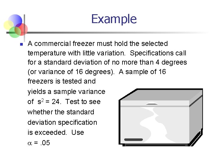
Example n A commercial freezer must hold the selected temperature with little variation. Specifications call for a standard deviation of no more than 4 degrees (or variance of 16 degrees). A sample of 16 freezers is tested and yields a sample variance of s 2 = 24. Test to see whether the standard deviation specification is exceeded. Use =. 05

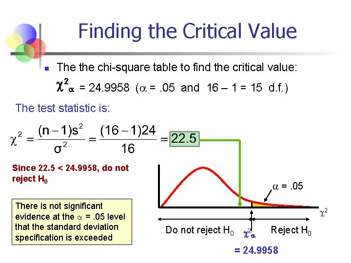
Finding the Critical Value n The the chi-square table to find the critical value: 2 = 24. 9958 ( =. 05 and 16 – 1 = 15 d. f. ) The test statistic is: Since 22. 5 < 24. 9958, do not reject H 0 There is not significant evidence at the =. 05 level that the standard deviation specification is exceeded =. 05 2 Do not reject H 0 2 Reject H 0 = 24. 9958

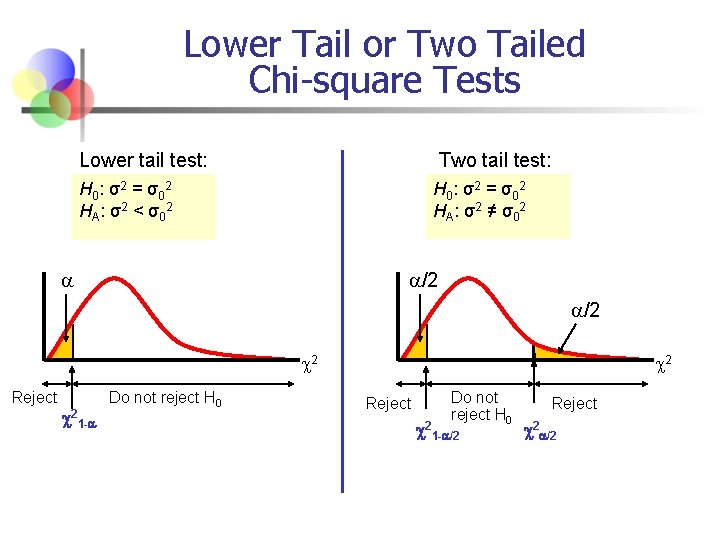
Lower Tail or Two Tailed Chi-square Tests Lower tail test: Two tail test: H 0 : σ2 = σ0 2 HA: σ2 < σ02 H 0 : σ2 = σ0 2 HA: σ2 ≠ σ02 /2 /2 2 Reject 21 - Do not reject H 0 2 Reject Do not reject H 0 21 - /2 Reject 2 /2

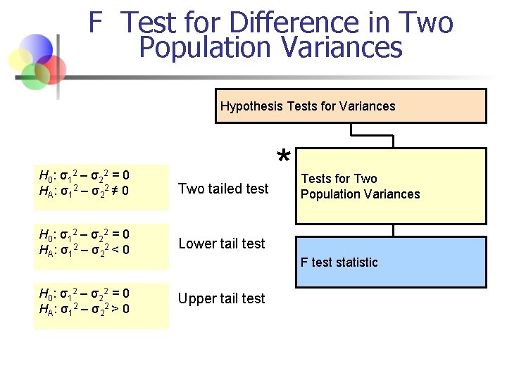
F Test for Difference in Two Population Variances Hypothesis Tests for Variances H 0 : σ1 2 – σ2 2 = 0 HA: σ12 – σ22 ≠ 0 Two tailed test H 0 : σ1 2 – σ2 2 = 0 HA: σ12 – σ22 < 0 Lower tail test H 0 : σ1 2 – σ2 2 = 0 HA: σ12 – σ22 > 0 Upper tail test * Tests for Two Population Variances F test statistic

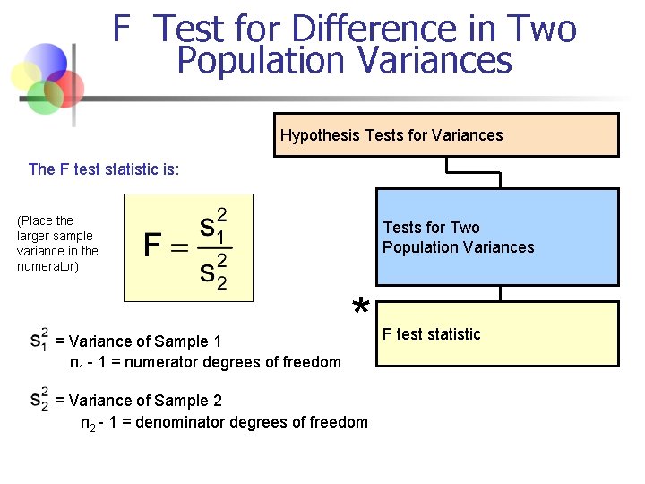
F Test for Difference in Two Population Variances Hypothesis Tests for Variances The F test statistic is: (Place the larger sample variance in the numerator) = Variance of Sample 1 n 1 - 1 = numerator degrees of freedom Tests for Two Population Variances * = Variance of Sample 2 n 2 - 1 = denominator degrees of freedom F test statistic

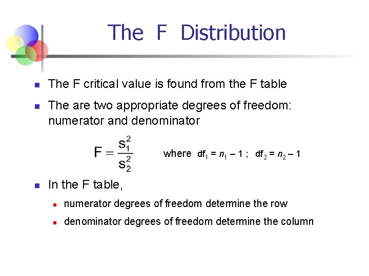
The F Distribution n n The F critical value is found from the F table The are two appropriate degrees of freedom: numerator and denominator where df 1 = n 1 – 1 ; df 2 = n 2 – 1 n In the F table, n numerator degrees of freedom determine the row n denominator degrees of freedom determine the column

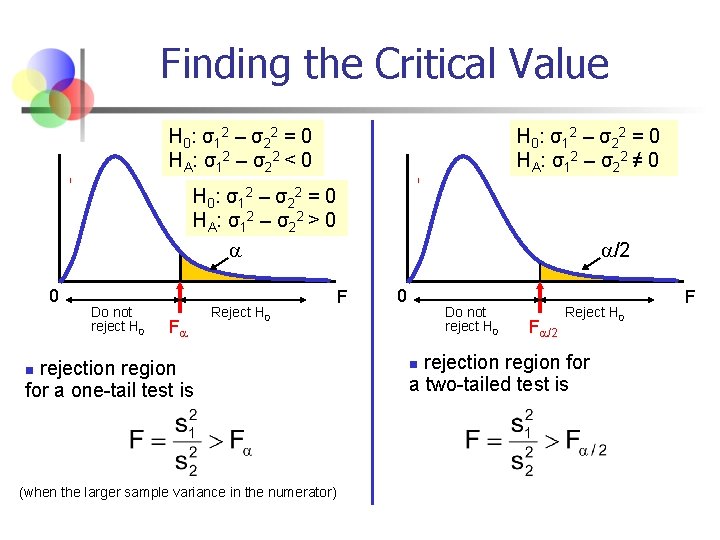
Finding the Critical Value H 0 : σ1 2 – σ2 2 = 0 HA: σ12 – σ22 < 0 H 0 : σ1 2 – σ2 2 = 0 HA: σ12 – σ22 ≠ 0 H 0 : σ1 2 – σ2 2 = 0 HA: σ12 – σ22 > 0 /2 0 Do not reject H 0 F Reject H 0 rejection region for a one-tail test is n (when the larger sample variance in the numerator) F 0 Do not reject H 0 F /2 Reject H 0 rejection region for a two-tailed test is n F

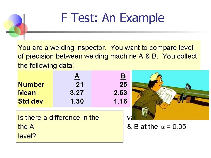
F Test: An Example You are a welding inspector. You want to compare level of precision between welding machine A & B. You collect the following data: A B Number 21 25 Mean 3. 27 2. 53 Std dev 1. 30 1. 16 Is there a difference in the A level? variances between & B at the = 0. 05

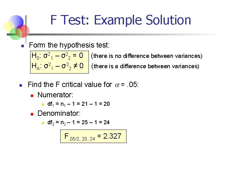
F Test: Example Solution n n Form the hypothesis test: H 0: σ21 – σ22 = 0 (there is no difference between variances) HA: σ21 – σ22 ≠ 0 (there is a difference between variances) Find the F critical value for =. 05: n Numerator: n n df 1 = n 1 – 1 = 20 Denominator: n df 2 = n 2 – 1 = 25 – 1 = 24 F. 05/2, 20, 24 = 2. 327

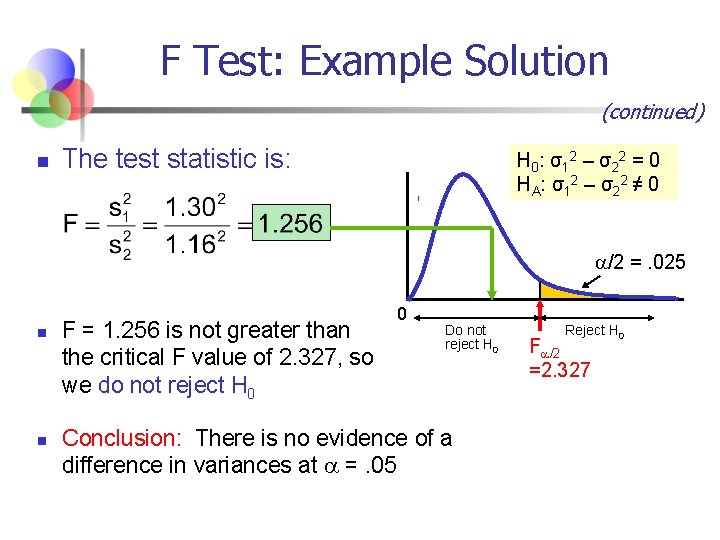
F Test: Example Solution (continued) n The test statistic is: H 0 : σ1 2 – σ2 2 = 0 HA: σ12 – σ22 ≠ 0 /2 =. 025 n n F = 1. 256 is not greater than the critical F value of 2. 327, so we do not reject H 0 0 Do not reject H 0 Conclusion: There is no evidence of a difference in variances at =. 05 Reject H 0 F /2 =2. 327