Estimation 4 Examples MLE and Unbiased estimation Example

Estimation 4: Examples, MLE and Unbiased estimation

Example The length of a shotgun barrel is measured with a ruler four times (units: in): 18. 438, 18. 440, 18. 468, 18. 437 Compute: a. b. c. d. e. The MLE sample mean: The unbiased sample sd: The unbiased standard error of the sample mean: Estimate the %relative (unbiased) standard deviation (with respect to the sample mean) Sketch and label the approximate (normal) sampling distribution using the sample mean as an estimate for the true mean and the sample standard error as an estimate for the true standard error.

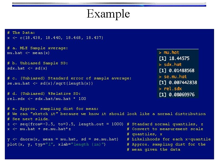
Example # The Data: x <- c(18. 438, 18. 440, 18. 468, 18. 437) # a. MLE Sample average: mu. hat <- mean(x) # b. Unbiased Sample SD: sdx. hat <- sd(x) # c. (Unbiased) Standard error of sample average: se. mu. hat <- sd(x)/sqrt(length(x)) # d. (Unbiased) %Relative SD: rel. sdx <- sdx. hat/mu. hat * 100 # # # z x e. Approx. sampling dist for mean: We can "sketch it" because we know it should look like a normal distribution See next slide… <- seq(from=-3. 5, to=3. 5, length. out = 1000) # Standard normal quantiles, z <- mu. hat + se. mu. hat*z # Convert to measurement scale # quantiles, x y <- dnorm(x, mean = mu. hat, sd = se. mu. hat) # Likelihoods for each x-quantile plot(x, y, typ="l", xlab="length (in)") # Approx. sampling dist for the # mean given the data

Example Approximate sampling distribution for the mean (barrel length) f. = 18. 446 in = ± 0. 007 in
- Slides: 4