ESTIMATING u AND d Binomial Distribution Derivation of

ESTIMATING u AND d Binomial Distribution Derivation of the Estimating Formula for u an d

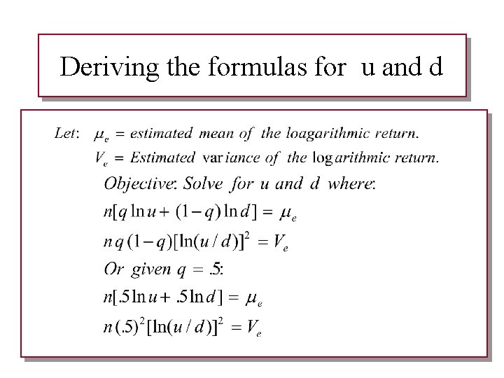
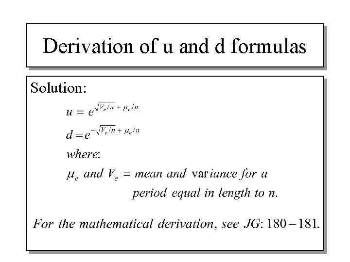
Estimating u and d The estimating equations for determining u and d are obtained by mathematically solving for the u and d values which make the statistical characteristics of a binomial distribution of the stock’s logarithmic returns equal to the characteristic's estimated value.

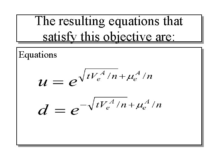
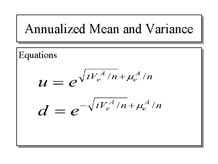
The resulting equations that satisfy this objective are: Equations

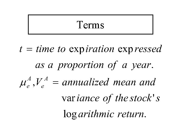
Terms

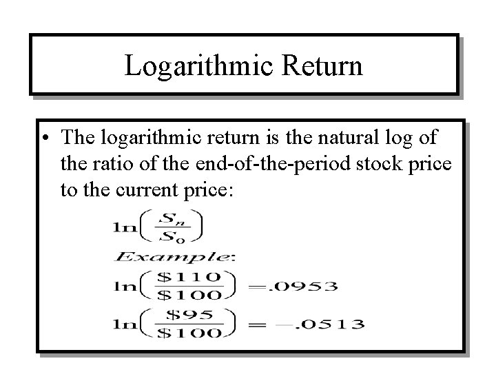
Logarithmic Return • The logarithmic return is the natural log of the ratio of the end-of-the-period stock price to the current price:

Annualized Mean and Variance • The annualized mean and variance are obtained by multiplying the estimated mean and variance of a given length (e. g, month) by the number of periods of that length in a year (e. g. , 12). • For an example, see JG, pp. 167 -168.

Example: JG, pp. 168 -169. • Using historical quarterly stock price data, suppose you estimate the stock’s quarterly mean and variance to be 0 and. 004209. • The annualized mean and variance would be 0 and. 016836. • If the number of subperiods for an expiration of one quarter (t=. 25) is n = 6, then u = 1. 02684 and d =. 9739.

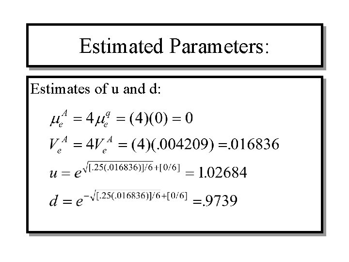
Estimated Parameters: Estimates of u and d:

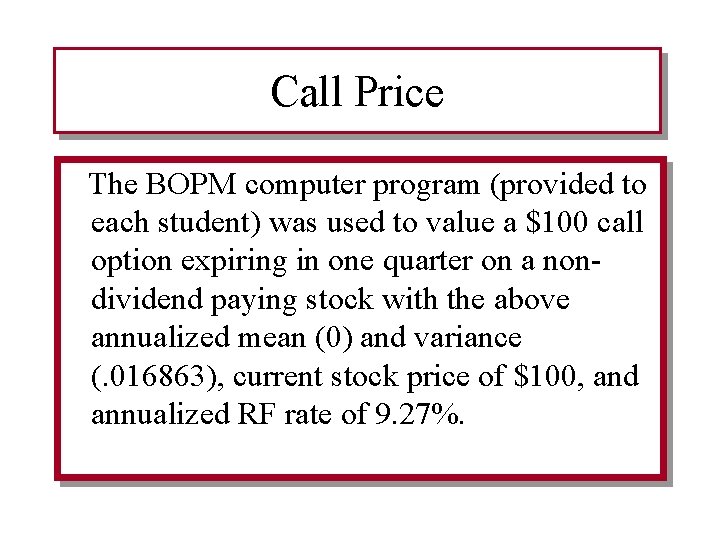
Call Price The BOPM computer program (provided to each student) was used to value a $100 call option expiring in one quarter on a nondividend paying stock with the above annualized mean (0) and variance (. 016863), current stock price of $100, and annualized RF rate of 9. 27%.

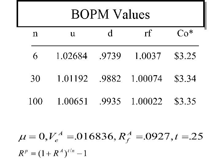
BOPM Values

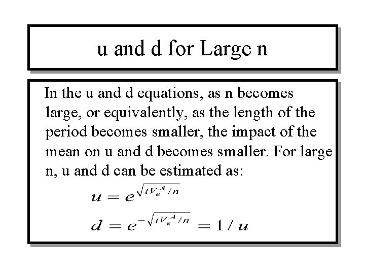
u and d for Large n In the u and d equations, as n becomes large, or equivalently, as the length of the period becomes smaller, the impact of the mean on u and d becomes smaller. For large n, u and d can be estimated as:

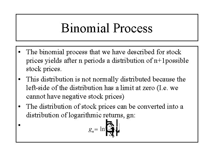
Binomial Process • The binomial process that we have described for stock prices yields after n periods a distribution of n+1 possible stock prices. • This distribution is not normally distributed because the left-side of the distribution has a limit at zero (I. e. we cannot have negative stock prices) • The distribution of stock prices can be converted into a distribution of logarithmic returns, gn: •

Binomial Process • The distribution of logarithmic returns can take on negative values and will be normally distributed if the probability of the stock increasing in one period (q) is. 5. • The next figure shows a distribution of stock prices and their corresponding logarithmic returns for the case in which u = 1. 1, d =. 95, and So = 100.

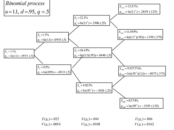
Binomial Process • Note: When n = 1, there are two possible prices and logarithmic returns:

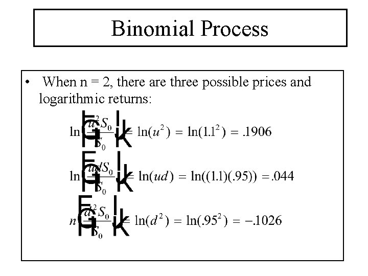
Binomial Process • When n = 2, there are three possible prices and logarithmic returns:

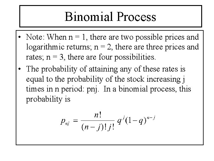
Binomial Process • Note: When n = 1, there are two possible prices and logarithmic returns; n = 2, there are three prices and rates; n = 3, there are four possibilities. • The probability of attaining any of these rates is equal to the probability of the stock increasing j times in n period: pnj. In a binomial process, this probability is

Binomial Distribution • Using the binomial probabilities, the expected value and variance of the logarithmic return after one period are. 022 and. 0054:

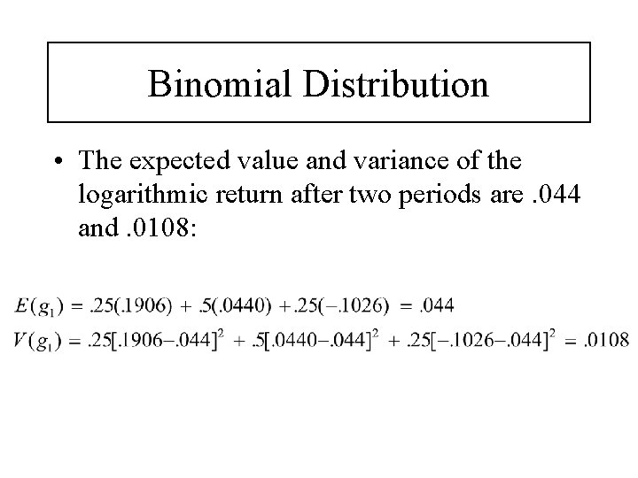
Binomial Distribution • The expected value and variance of the logarithmic return after two periods are. 044 and. 0108:

Binomial Distribution • Note: The parameter values (expected value and variance) after n periods are equal to the parameter values for one period time the number of periods:

Binomial Distribution • Note: The expected value and variance of the logarithmic return are also equal to

Deriving the formulas for u and d The estimating equations for determining u and d are obtained by mathematically solving for the u and d values which make the expected value and variance of a binomial distribution of the stock’s logarithmic returns equal to the characteristic's estimated value.

Deriving the formulas for u and d

Derivation of u and d formulas Solution:

Annualized Mean and Variance Equations