Estimating Timing Profiles for Simulation of Embedded Systems

Estimating Timing Profiles for Simulation of Embedded Systems Andrew H. Chan May 15, 2009

Introduction o o Timing estimation Timing and Concurrency n n o Many parts working together Need to be aware of timing characteristics Given hardware, software and control flow, estimate execution time

Motivation o Access Point Event Simulation of Legacy Embedded Software Systems (APES) n n o o Discrete event model in Ptolemy Needs timing estimates of code fragments Easier/less expensive to simulate in software without maintaining actual hardware Might not have direct access to hardware

Motivation o o o Explore timing behavior of hardware Guided testing to assess timing characteristics Simplify problem by deciding on both software and hardware

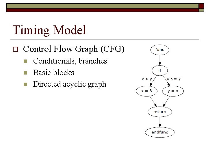
Timing Model o Control Flow Graph (CFG) n n n Conditionals, branches Basic blocks Directed acyclic graph

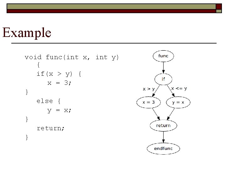
Example void func(int x, int y) { if(x > y) { x = 3; } else { y = x; } return; }

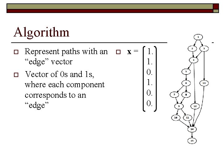
Algorithm o o Represent paths with an “edge” vector Vector of 0 s and 1 s, where each component corresponds to an “edge” o x= 1. 1. 0. 0.

Algorithm o Calculate 2 -barycentric spanner n n o o Good representative set of basis paths Every path can be represented by a linear combination with coeff less than 2 Sample on these paths to obtain timing information Only get total path execution times n No execution times for individual basic blocks

Algorithm o o o B is a matrix with basis vectors as rows v is a vector of the average execution times for the basis vectors w is the “edge weight” vector Bw = v w = B-1 v Estimate for path x n w. Tx = estimated time

Algorithm o o Estimate “edge” weights Path lengths are more important n n Not all edges are assigned accurate weights, but it doesn’t matter Only the overall path length matters

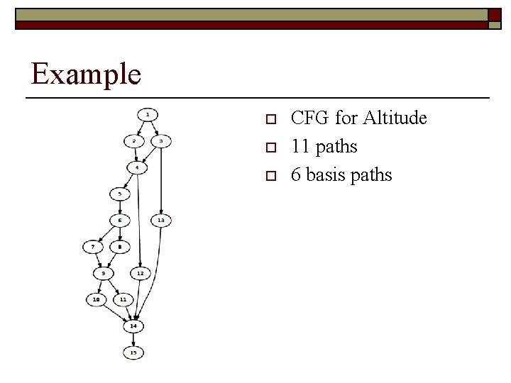
Example o o o CFG for Altitude 11 paths 6 basis paths

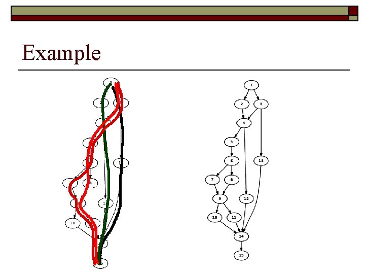
Example

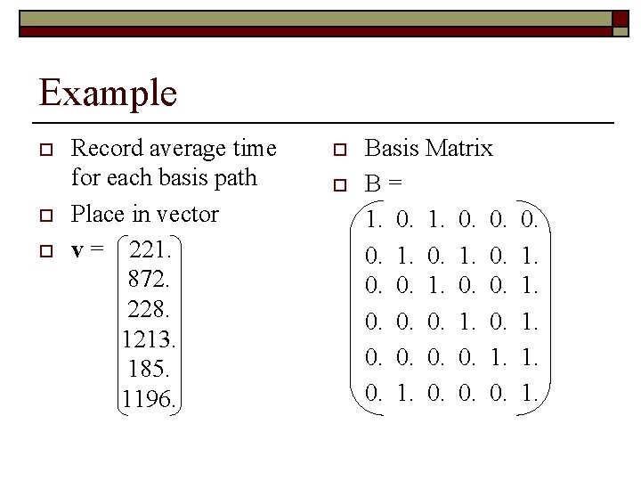
Example o o o Record average time for each basis path Place in vector v = 221. 872. 228. 1213. 185. 1196. o o Basis Matrix B= 1. 0. 0. 0. 1. 1. 1.

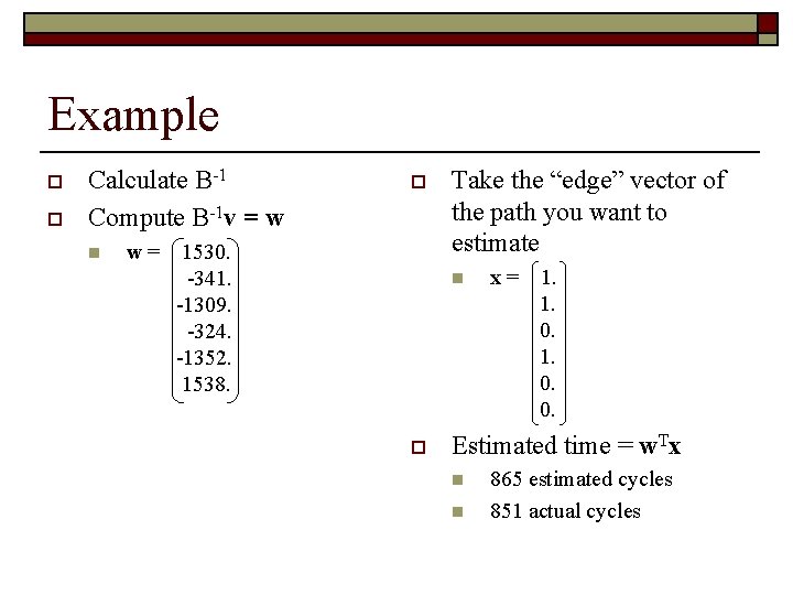
Example o o Calculate B-1 Compute B-1 v = w n w= o 1530. -341. -1309. -324. -1352. 1538. Take the “edge” vector of the path you want to estimate n o x= 1. 1. 0. 0. Estimated time = w. Tx n n 865 estimated cycles 851 actual cycles

Implementation o o o Sim. It ARM simulator CREST: branch coverage CIL: C front-end, instrumentation Yices: satisfiability solver Sci. Py and Numpy

Implementation o Sim. It ARM 2. 1 simulator n n n Cycle-accurate simulator for the Strong. ARM microprocessor ARM V 4 instruction set architecture 206 MHz processor

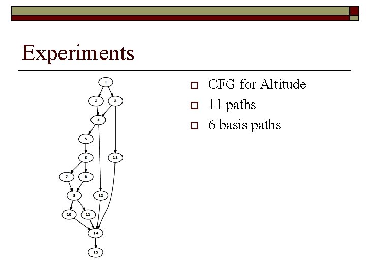
Experiments o o o CFG for Altitude 11 paths 6 basis paths

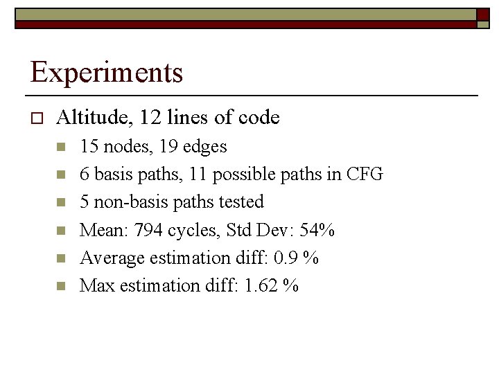
Experiments o Altitude, 12 lines of code n n n 15 nodes, 19 edges 6 basis paths, 11 possible paths in CFG 5 non-basis paths tested Mean: 794 cycles, Std Dev: 54% Average estimation diff: 0. 9 % Max estimation diff: 1. 62 %

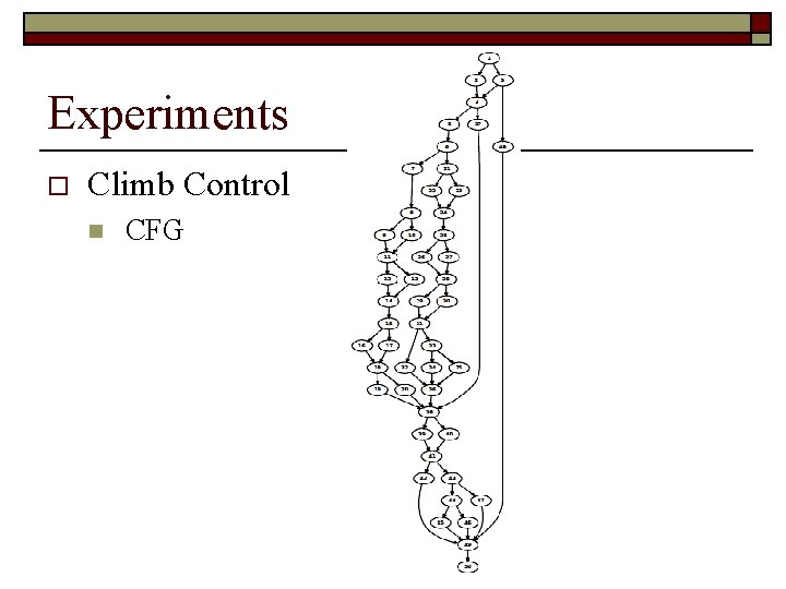
Experiments o Climb Control n CFG

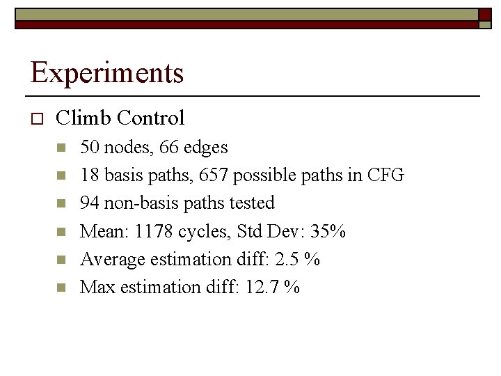
Experiments o Climb Control n n n 50 nodes, 66 edges 18 basis paths, 657 possible paths in CFG 94 non-basis paths tested Mean: 1178 cycles, Std Dev: 35% Average estimation diff: 2. 5 % Max estimation diff: 12. 7 %

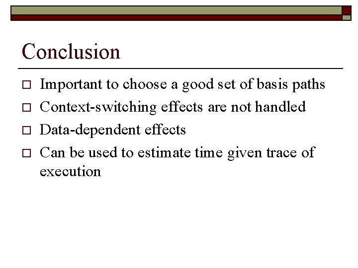
Conclusion o o Important to choose a good set of basis paths Context-switching effects are not handled Data-dependent effects Can be used to estimate time given trace of execution

Questions?