Estimating the Variance of the Error Terms The

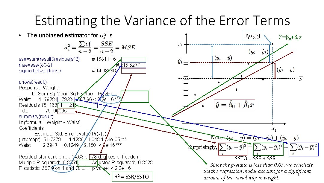
Estimating the Variance of the Error Terms • The unbiased estimator for σε 2 is Pi(xi, yi) Y=β 0+β 1 x yi sse=sum(result$residuals^2) mse=sse/(80 -2) sigma. hat=sqrt(mse) * # 16811. 16 * # 215. 5277 # 14. 68086 anova(result) Response: Weight Df Sum Sq Mean Sq F value Pr(>F) Waist 1 79284 367. 86 < 2. 2 e-16 *** Residuals 78 16811 216 Total 79 96095 summary(result) lm(formula = Weight ~ Waist) Coefficients: Estimate Std. Error t value Pr(>|t|) (Intercept) -51. 7279 11. 1288 -4. 648 1. 34 e-05 *** Waist 2. 3947 0. 1249 19. 180 < 2 e-16 *** Residual standard error: 14. 68 on 78 degrees of freedom Multiple R-squared: 0. 8251, Adjusted R-squared: 0. 8228 F-statistic: 367. 9 on 1 and 78 DF, p-value: < 2. 2 e-16 R 2 = SSR/SSTO * * * y * * * xi SSTO = SSE + SSR Since the p-vlaue is less than 0. 05, we conclude the regression model account for a significant 1 amount of the variability in weight.

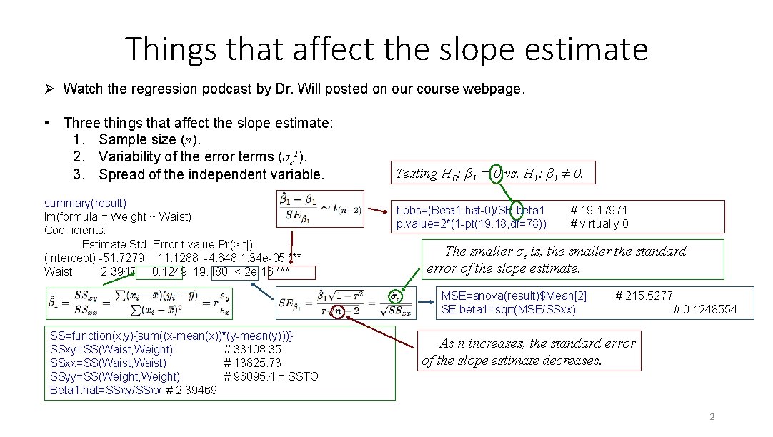
Things that affect the slope estimate Ø Watch the regression podcast by Dr. Will posted on our course webpage. • Three things that affect the slope estimate: 1. Sample size (n). 2. Variability of the error terms (σε 2). 3. Spread of the independent variable. summary(result) lm(formula = Weight ~ Waist) Coefficients: Estimate Std. Error t value Pr(>|t|) (Intercept) -51. 7279 11. 1288 -4. 648 1. 34 e-05 *** Waist 2. 3947 0. 1249 19. 180 < 2 e-16 *** Testing H 0: β 1 = 0 vs. H 1: β 1 ≠ 0. t. obs=(Beta 1. hat-0)/SE. beta 1 p. value=2*(1 -pt(19. 18, df=78)) # 19. 17971 # virtually 0 The smaller σε is, the smaller the standard error of the slope estimate. MSE=anova(result)$Mean[2] SE. beta 1=sqrt(MSE/SSxx) SS=function(x, y){sum((x-mean(x))*(y-mean(y)))} SSxy=SS(Waist, Weight) # 33108. 35 SSxx=SS(Waist, Waist) # 13825. 73 SSyy=SS(Weight, Weight) # 96095. 4 = SSTO Beta 1. hat=SSxy/SSxx # 2. 39469 # 215. 5277 # 0. 1248554 As n increases, the standard error of the slope estimate decreases. 2

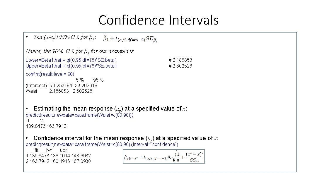
Confidence Intervals • The (1 -α)100% C. I. for β 1: Hence, the 90% C. I. for β 1 for our example is Lower=Beta 1. hat – qt(0. 95, df=78)*SE. beta 1 Upper=Beta 1. hat + qt(0. 95, df=78)*SE. beta 1 # 2. 186853 # 2. 602528 confint(result, level=. 90) 5% 95 % (Intercept) -70. 253184 -33. 202619 Waist 2. 186853 2. 602528 • Estimating the mean response (μy) at a specified value of x: predict(result, newdata=data. frame(Waist=c(80, 90))) 1 2 139. 8473 163. 7942 • Confidence interval for the mean response (μy) at a specified value of x: predict(result, newdata=data. frame(Waist=c(80, 90)), interval=”confidence”) fit lwr upr 1 139. 8473 136. 0014 143. 6932 2 163. 7942 160. 4946 167. 0938

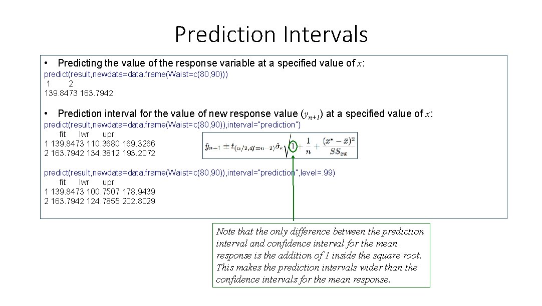
Prediction Intervals • Predicting the value of the response variable at a specified value of x: predict(result, newdata=data. frame(Waist=c(80, 90))) 1 2 139. 8473 163. 7942 • Prediction interval for the value of new response value (yn+1) at a specified value of x: predict(result, newdata=data. frame(Waist=c(80, 90)), interval=”prediction”) fit lwr upr 1 139. 8473 110. 3680 169. 3266 2 163. 7942 134. 3812 193. 2072 predict(result, newdata=data. frame(Waist=c(80, 90)), interval=”prediction”, level=. 99) fit lwr upr 1 139. 8473 100. 7507 178. 9439 2 163. 7942 124. 7855 202. 8029 Note that the only difference between the prediction interval and confidence interval for the mean response is the addition of 1 inside the square root. This makes the prediction intervals wider than the confidence intervals for the mean response.

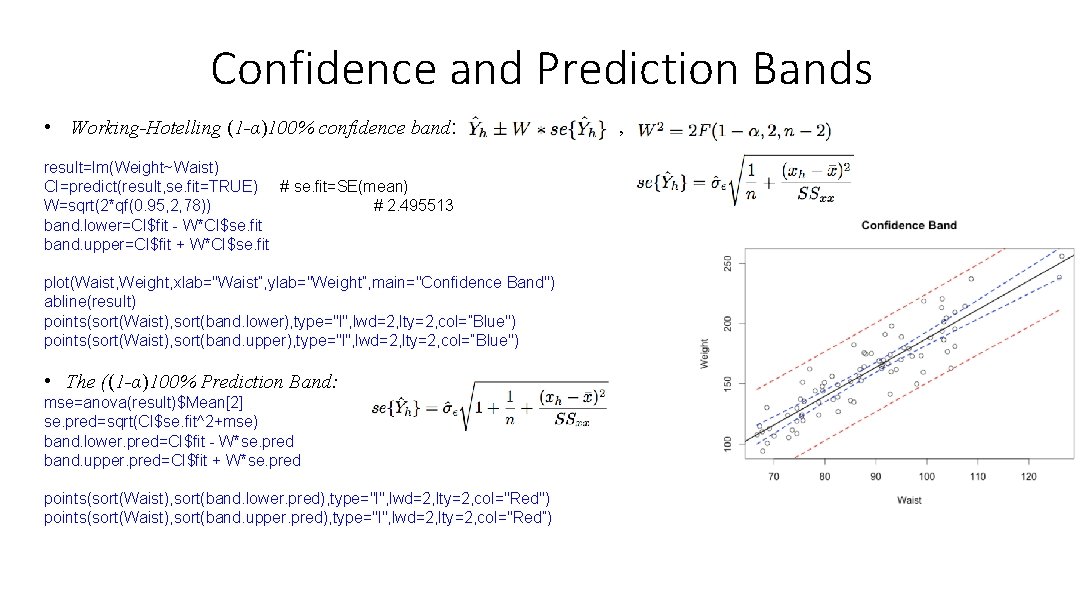
Confidence and Prediction Bands • Working-Hotelling (1 -α)100% confidence band: result=lm(Weight~Waist) CI=predict(result, se. fit=TRUE) # se. fit=SE(mean) W=sqrt(2*qf(0. 95, 2, 78)) # 2. 495513 band. lower=CI$fit - W*CI$se. fit band. upper=CI$fit + W*CI$se. fit plot(Waist, Weight, xlab="Waist”, ylab="Weight”, main="Confidence Band") abline(result) points(sort(Waist), sort(band. lower), type="l", lwd=2, lty=2, col=”Blue") points(sort(Waist), sort(band. upper), type="l", lwd=2, lty=2, col=”Blue") • The ((1 -α)100% Prediction Band: mse=anova(result)$Mean[2] se. pred=sqrt(CI$se. fit^2+mse) band. lower. pred=CI$fit - W*se. pred band. upper. pred=CI$fit + W*se. pred points(sort(Waist), sort(band. lower. pred), type="l", lwd=2, lty=2, col="Red") points(sort(Waist), sort(band. upper. pred), type="l", lwd=2, lty=2, col="Red”) ,

Tests for Correlations • Testing H 0: ρ = 0 vs. H 1: ρ ≠ 0. cor(Waist, Weight) # Computes the Pearson correlation coefficient, r 0. 9083268 cor. test(Waist, Weight, conf. level=. 99) # Tests Ho: rho=0 and also constructs C. I. for rho Pearson's product-moment correlation data: Waist and Weight Note that the results are exactly t = 19. 1797, df = 78, p-value < 2. 2 e-16 the same as what we got when alternative hypothesis: true correlation is not equal to 0 testing H 0: β 1 = 0 vs. H 1: β 1 ≠ 0. 99 percent confidence interval: 0. 8409277 0. 9479759 • Testing H 0: ρ = 0 vs. H 1: ρ ≠ 0 using the (Nonparametric) Spearman’s method. cor. test(Waist, Weight, method="spearman") # Test of independence using the Spearman's rank correlation rho # Spearman Rank correlation data: Waist and Weight S = 8532, p-value < 2. 2 e-16 alternative hypothesis: true rho is not equal to 0 sample estimates: rho 0. 9 6

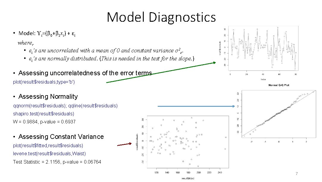
Model Diagnostics • Model: Yi=(β 0+β 1 xi) + εi where, • εi’s are uncorrelated with a mean of 0 and constant variance σ2ε. • εi’s are normally distributed. (This is needed in the test for the slope. ) • Assessing uncorrelatedness of the error terms plot(result$residuals, type='b') • Assessing Normality qqnorm(result$residuals); qqline(result$residuals) shapiro. test(result$residuals) W = 0. 9884, p-value = 0. 6937 • Assessing Constant Variance plot(result$fitted, result$residuals) levene. test(result$residuals, Waist) Test Statistic = 2. 1156, p-value = 0. 06764 7