ESTIMATING THE DOSERESPONSE FUNCTION THROUGH THE GLM APPROACH

ESTIMATING THE DOSE-RESPONSE FUNCTION THROUGH THE GLM APPROACH Barbara Guardabascio, Marco Ventura Italian National Institute of Statistics 7 th June 2013, Potsdam 1

Outline of the talk Ø Motivations; Ø literature references; Ø our contribution to the topic; Ø the econometrics of the dose-response; Ø how to implement the dose-response; Ø our programs; Ø applications. 2

Motivations Ø Main question: how effective are public policy programs with continuous treatment exposure? Ø Fundamental problem: treated individuals are self-selected and not randomly. Treatment is not randomly assigned Ø (possible) solution: estimating a dose-response function 3

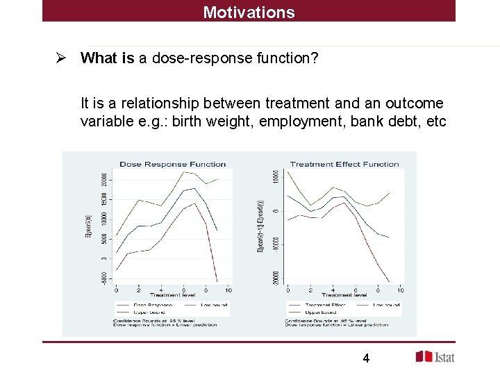
Motivations Ø What is a dose-response function? It is a relationship between treatment and an outcome variable e. g. : birth weight, employment, bank debt, etc 4

Motivations Ø How can we estimate a dose-response function? It can be estimated by using the Generalized Propensity Score (GPS) 5

Literature references 1. Propensity Score for binary treatments: Rosenbaum and Rubin (1983), (1984) 2. for categorical treatment variables: Imbens (2000), Lechner (2001) 3. Generalized Propensity Score for continuous treatments: Hirano and Imbens, 2004; Imai and Van Dyk (2004) 6

Our contribution Ø Ad hoc programs have been provided to STATA users (Bia and Mattei, 2008), but … … these programs contemplate only Normal distribution of the treatment variable (gpscore. ado and doseresponse. ado) Ø We provide new programs to accommodate other distributions, not Normal. (gpscore 2. ado and doseresponse 2. ado) 7

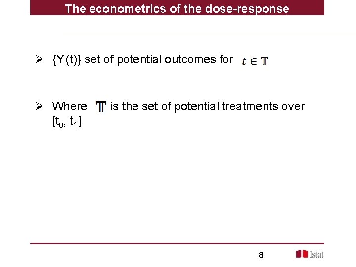
The econometrics of the dose-response Ø {Yi(t)} set of potential outcomes for Ø Where [t 0, t 1] is the set of potential treatments over 8

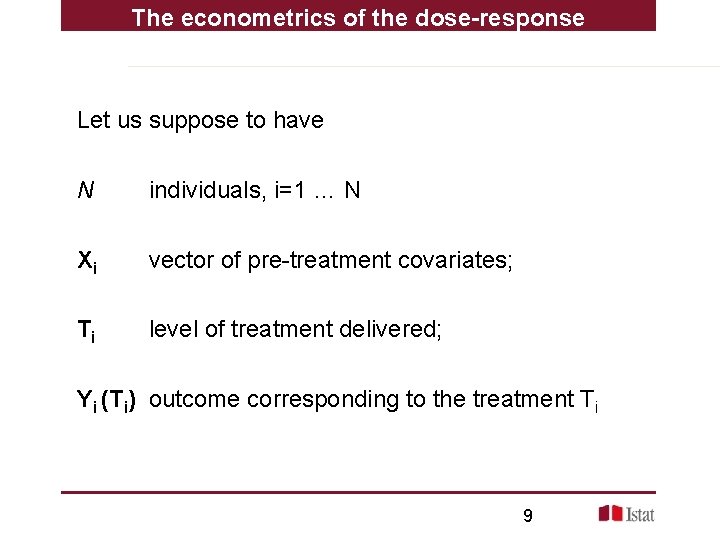
The econometrics of the dose-response Let us suppose to have N individuals, i=1 … N Xi vector of pre-treatment covariates; Ti level of treatment delivered; Yi (Ti) outcome corresponding to the treatment Ti 9

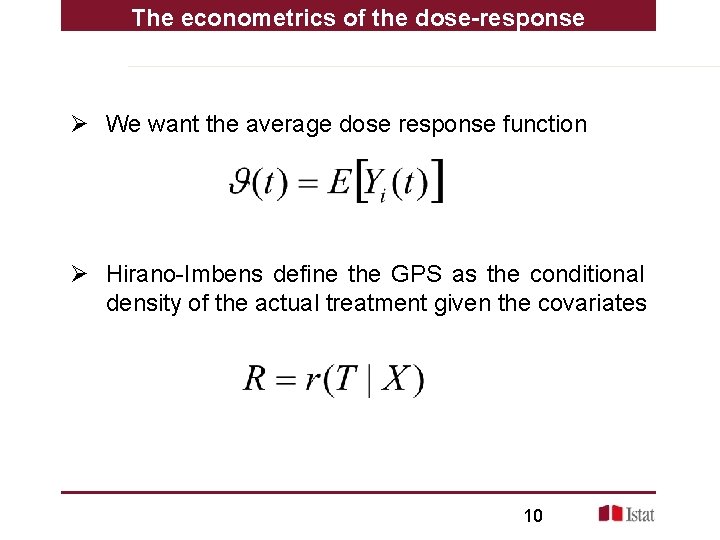
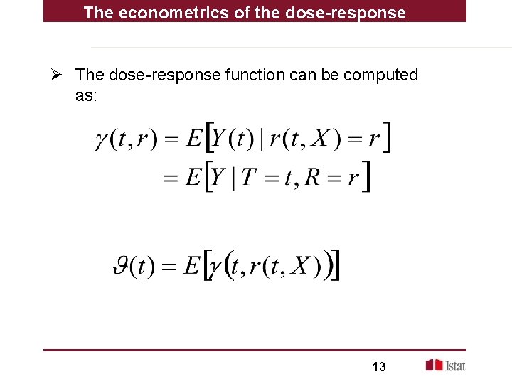
The econometrics of the dose-response Ø We want the average dose response function Ø Hirano-Imbens define the GPS as the conditional density of the actual treatment given the covariates 10

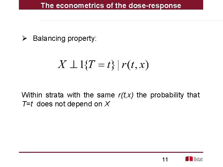
The econometrics of the dose-response Ø Balancing property: Within strata with the same r(t, x) the probability that T=t does not depend on X 11

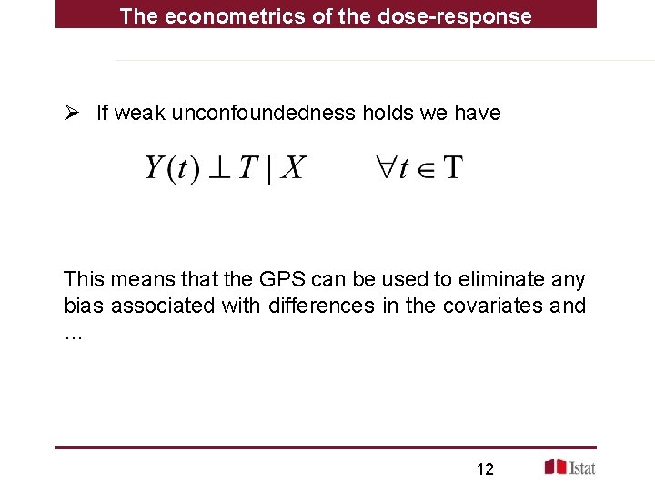
The econometrics of the dose-response Ø If weak unconfoundedness holds we have This means that the GPS can be used to eliminate any bias associated with differences in the covariates and … 12

The econometrics of the dose-response Ø The dose-response function can be computed as: 13

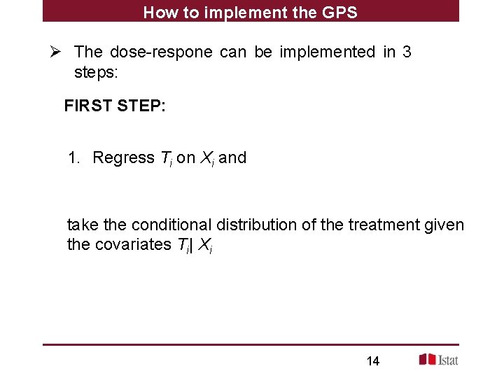
How to implement the GPS Ø The dose-respone can be implemented in 3 steps: FIRST STEP: 1. Regress Ti on Xi and take the conditional distribution of the treatment given the covariates Ti| Xi 14

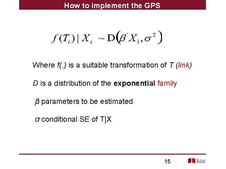
How to implement the GPS Where f(. ) is a suitable transformation of T (link) D is a distribution of the exponential family β parameters to be estimated σ conditional SE of T|X 15

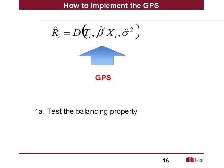
How to implement the GPS 1 a. Test the balancing property 16

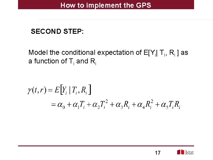
How to implement the GPS SECOND STEP: Model the conditional expectation of E[Yi| Ti, Ri ] as a function of Ti and Ri 17

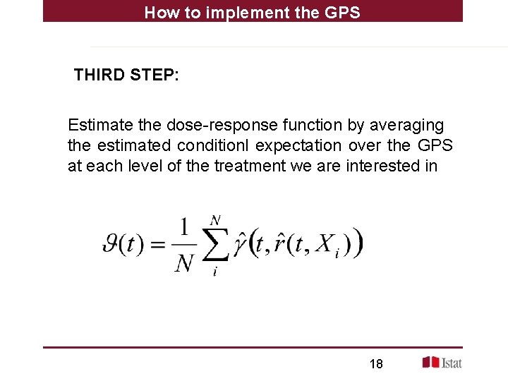
How to implement the GPS THIRD STEP: Estimate the dose-response function by averaging the estimated conditionl expectation over the GPS at each level of the treatment we are interested in 18

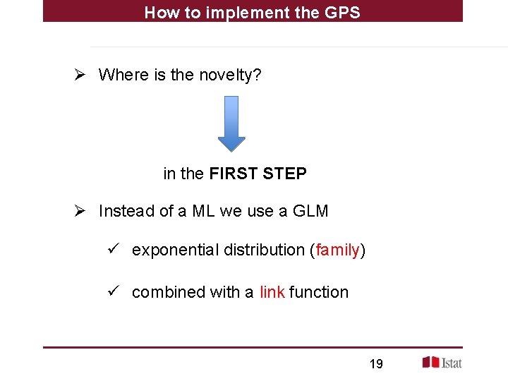
How to implement the GPS Ø Where is the novelty? in the FIRST STEP Ø Instead of a ML we use a GLM ü exponential distribution (family) ü combined with a link function 19

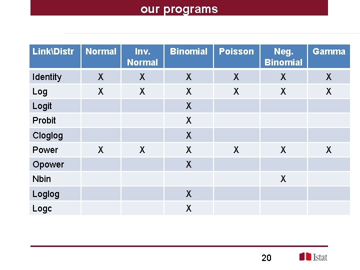
our programs LinkDistr Normal Inv. Normal Binomial Poisson Neg. Binomial Gamma Identity X X X Log X X X X X Logit X Probit X Cloglog X Power Opower X X Nbin X Loglog X Logc X 20

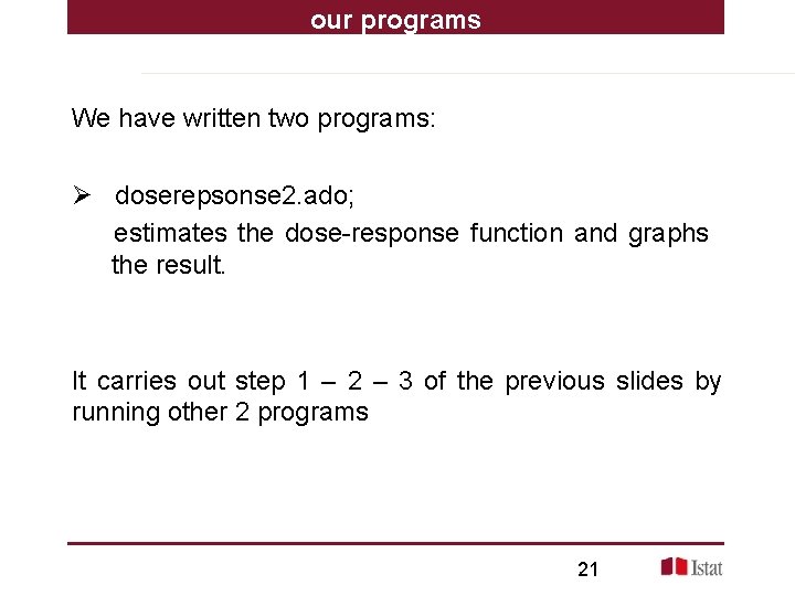
our programs We have written two programs: Ø doserepsonse 2. ado; estimates the dose-response function and graphs the result. It carries out step 1 – 2 – 3 of the previous slides by running other 2 programs 21

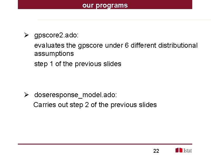
our programs Ø gpscore 2. ado: evaluates the gpscore under 6 different distributional assumptions step 1 of the previous slides Ø doseresponse_model. ado: Carries out step 2 of the previous slides 22

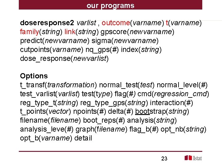
our programs doseresponse 2 varlist , outcome(varname) t(varname) family(string) link(string) gpscore(newvarname) predict(newvarname) sigma(newvarname) cutpoints(varname) nq_gps(#) index(string) dose_response(newvarlist) Options t_transf(transformation) normal_test(test) normal_level(#) test_varlist(varlist) test(type) flag(#) cmd(regression_cmd) reg_type_t(string) reg_type_gps(string) interaction(#) t_points(vector) npoints(#) delta(#) bootstrap(string) filename(filename) boot_reps(#) analysis(string) analysis_leve(#) graph(filename) flag_b(#) opt_nb(string) opt_b(varname) detail 23

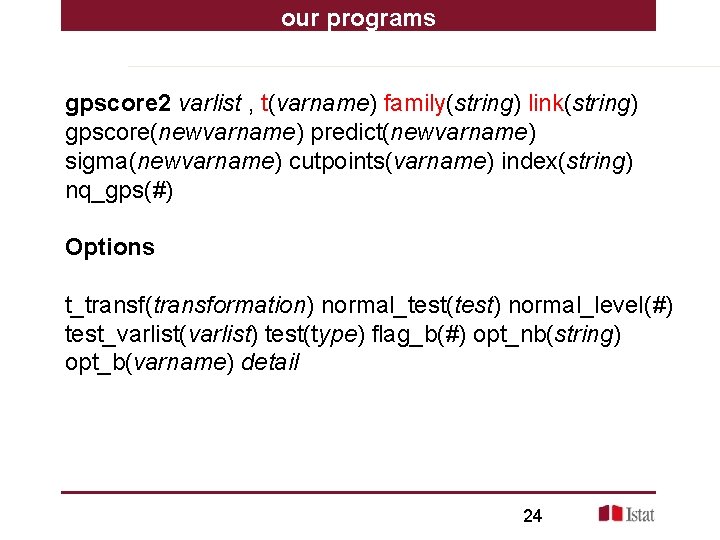
our programs gpscore 2 varlist , t(varname) family(string) link(string) gpscore(newvarname) predict(newvarname) sigma(newvarname) cutpoints(varname) index(string) nq_gps(#) Options t_transf(transformation) normal_test(test) normal_level(#) test_varlist(varlist) test(type) flag_b(#) opt_nb(string) opt_b(varname) detail 24

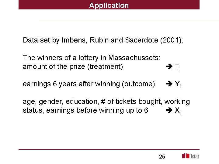
Application Data set by Imbens, Rubin and Sacerdote (2001); The winners of a lottery in Massachussets: amount of the prize (treatment) Ti earnings 6 years after winning (outcome) Yi age, gender, education, # of tickets bought, working status, earnings before winning up to 6 Xi 25

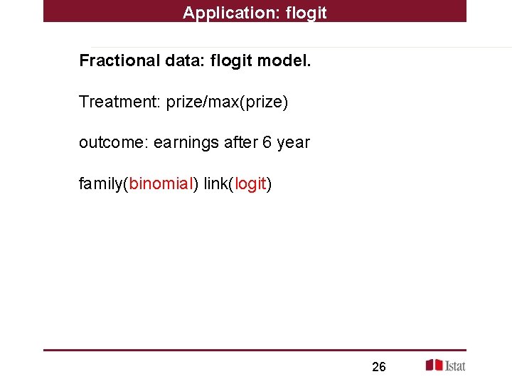
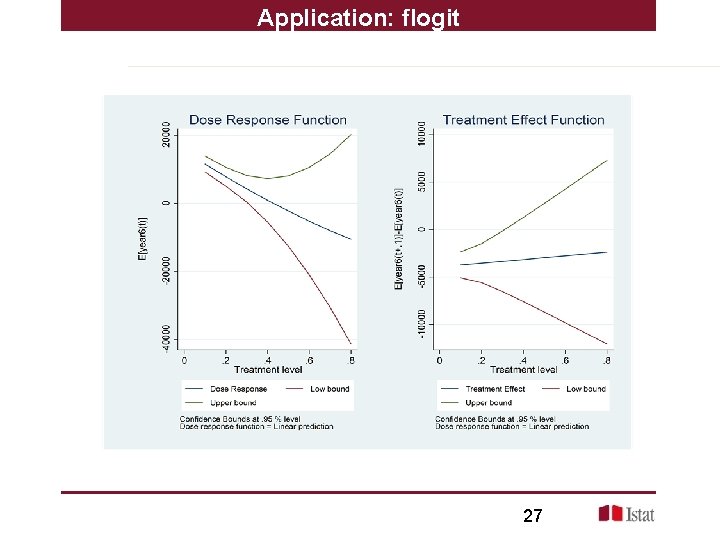
Application: flogit Fractional data: flogit model. Treatment: prize/max(prize) outcome: earnings after 6 year family(binomial) link(logit) 26

Application: flogit 27

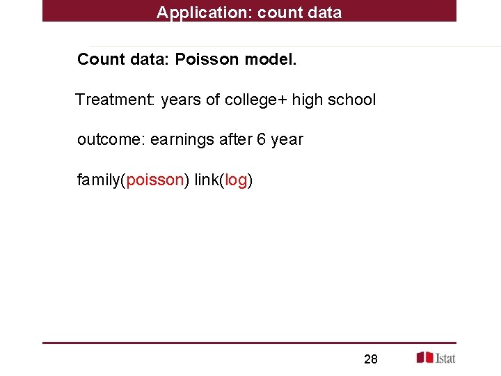
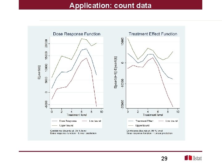
Application: count data Count data: Poisson model. Treatment: years of college+ high school outcome: earnings after 6 year family(poisson) link(log) 28

Application: count data 29

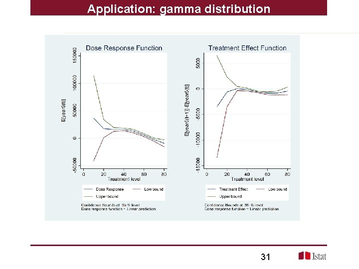
Application: gamma distribution Gamma distribution: Treatment: age outcome: earnings after 6 year family(gamma) link(log) 30

Application: gamma distribution 31