Estimating Population Parameters Based on a Sample Population

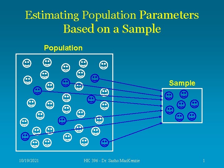
Estimating Population Parameters Based on a Sample Population Sample 10/19/2021 HK 396 - Dr. Sasho Mac. Kenzie 1

Why Estimate? • It is often not feasible (lack of time and money) to measure an entire population. • Therefore, a researcher must select a representative sample from the population and make estimations. • This general principle is used frequently in research and is known as statistical inference. 10/19/2021 HK 396 - Dr. Sasho Mac. Kenzie 2

Estimating a Population Mean • Researchers often want to know the mean of a population. • E. g. , Health Canada, may want to understand obesity trends over the next 10 years. • The first step would be to measure obesity in the population on an annual basis (measure BMI). • Researchers cannot measure all 20 million adult Canadians every year. • Each year a random sample is measured and used to estimate the entire population. 10/19/2021 HK 396 - Dr. Sasho Mac. Kenzie 3

Sampling Error • It is unlikely that the sample will have exactly the same mean as the entire population. • Sampling error is the amount of error in the estimate of a population parameter that is based on a sample statistic. • Therefore, Health Canada needs to determine how accurate the mean BMI of the sample is and what the odds are that it is different from the population mean by a given amount. 10/19/2021 HK 396 - Dr. Sasho Mac. Kenzie 4

Standard Error of the Mean (SEM) • Standard error of the mean is a numeric value that indicates the amount of error that may occur when estimating a population mean. • The estimation of the population mean is always an educated guess and is accompanied by a probability statement. • I. e. , upper and lower limits can be set around the estimated mean and the chance of the true mean falling in this range can be stated as a probability such as, 5 out of 100 times, or p=. 05 10/19/2021 HK 396 - Dr. Sasho Mac. Kenzie 5

Understanding SEM • Consider the following theoretical exercise. • Take 100 random samples (N=400) of the Canadian adult population and find the mean BMI of each sample. • This means measuring 400 people and getting a mean BMI, then repeating the process 100 times. • This generates 100 estimates of the population mean. 10/19/2021 HK 396 - Dr. Sasho Mac. Kenzie 6

Understanding SEM • The majority of the 100 sample means will cluster around the true mean of the population. • However, some will also stray further from the true population mean. • The sample means will form a normal distribution in the same way individual BMI measurements within a sample form a normal distribution. • The standard deviation of the 100 sample means is the SEM. 10/19/2021 HK 396 - Dr. Sasho Mac. Kenzie 7

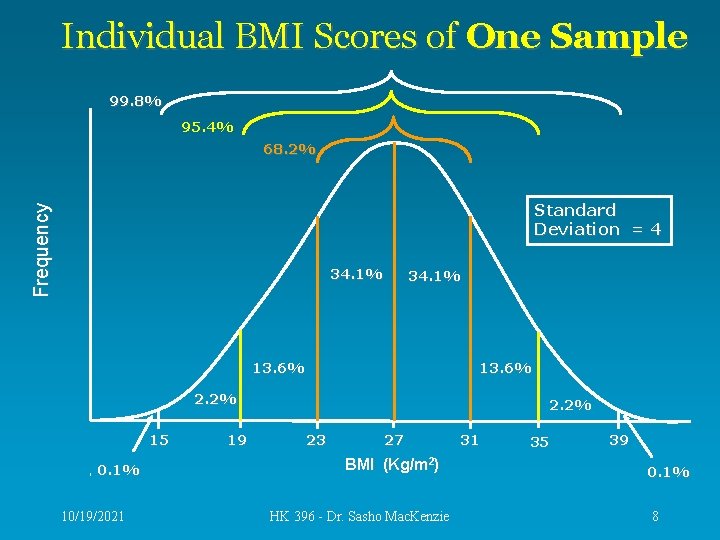
Individual BMI Scores of One Sample 99. 8% 95. 4% 68. 2% Frequency Standard Deviation = 4 34. 1% 13. 6% 2. 2% 15 0. 1% 10/19/2021 19 2. 2% 23 27 BMI (Kg/m 2) HK 396 - Dr. Sasho Mac. Kenzie 31 35 39 0. 1% 8

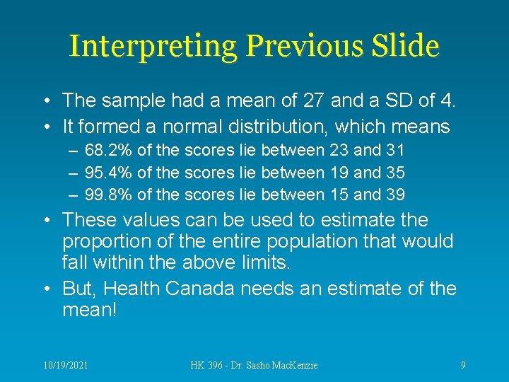
Interpreting Previous Slide • The sample had a mean of 27 and a SD of 4. • It formed a normal distribution, which means – – – 68. 2% of the scores lie between 23 and 31 95. 4% of the scores lie between 19 and 35 99. 8% of the scores lie between 15 and 39 • These values can be used to estimate the proportion of the entire population that would fall within the above limits. • But, Health Canada needs an estimate of the mean! 10/19/2021 HK 396 - Dr. Sasho Mac. Kenzie 9

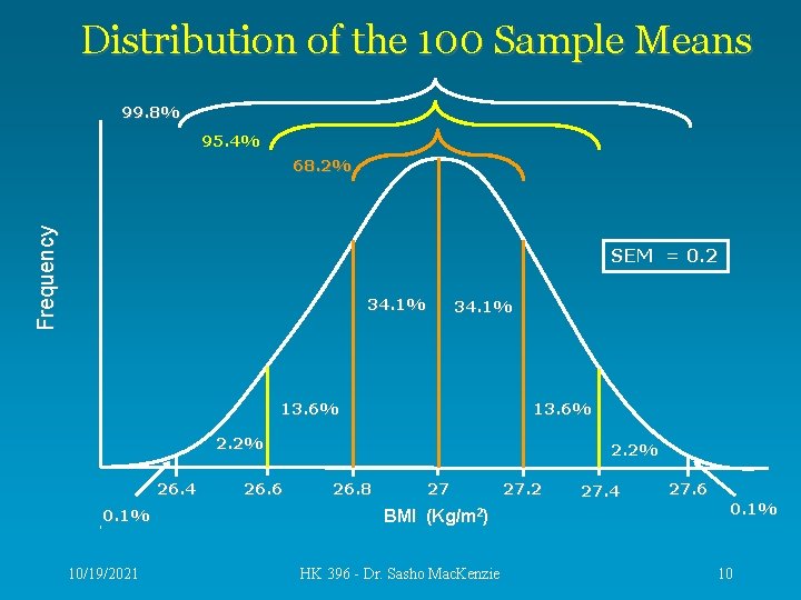
Distribution of the 100 Sample Means 99. 8% 95. 4% Frequency 68. 2% SEM = 0. 2 34. 1% 13. 6% 2. 2% 26. 4 0. 1% 10/19/2021 26. 6 2. 2% 26. 8 27 BMI (Kg/m 2) HK 396 - Dr. Sasho Mac. Kenzie 27. 2 27. 4 27. 6 0. 1% 10

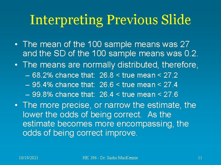
Interpreting Previous Slide • The mean of the 100 sample means was 27 and the SD of the 100 sample means was 0. 2. • The means are normally distributed, therefore, – 68. 2% chance that: 26. 8 < true mean < 27. 2 – 95. 4% chance that: 26. 6 < true mean < 27. 4 – 99. 8% chance that: 26. 4 < true mean < 27. 6 • The more precise, or narrow the estimate, the lower the odds of being correct. As the estimate becomes more encompassing, the odds of being correct improve. 10/19/2021 HK 396 - Dr. Sasho Mac. Kenzie 11

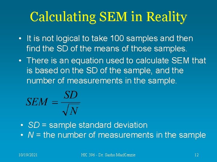
Calculating SEM in Reality • It is not logical to take 100 samples and then find the SD of the means of those samples. • There is an equation used to calculate SEM that is based on the SD of the sample, and the number of measurements in the sample. • SD = sample standard deviation • N = the number of measurements in the sample 10/19/2021 HK 396 - Dr. Sasho Mac. Kenzie 12

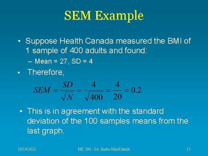
SEM Example • Suppose Health Canada measured the BMI of 1 sample of 400 adults and found: – Mean = 27, SD = 4 • Therefore, • This is in agreement with the standard deviation of the 100 samples means from the last graph. 10/19/2021 HK 396 - Dr. Sasho Mac. Kenzie 13

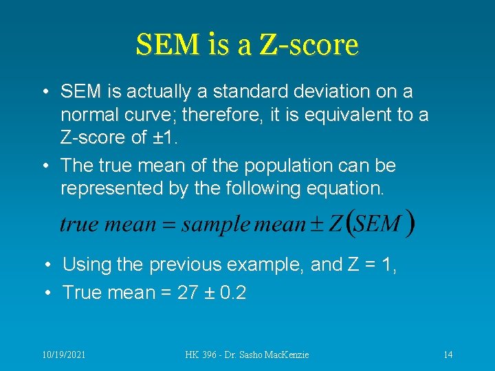
SEM is a Z-score • SEM is actually a standard deviation on a normal curve; therefore, it is equivalent to a Z-score of ± 1. • The true mean of the population can be represented by the following equation. • Using the previous example, and Z = 1, • True mean = 27 ± 0. 2 10/19/2021 HK 396 - Dr. Sasho Mac. Kenzie 14

Level of Confidence • A level of confidence (LOC) is a percentage figure that establishes the probability that a statement is correct. • It is based on the characteristics of the normal curve. • Using the example from the last slide, • Health Canada can conclude that the mean BMI for adults, 27 ± 0. 2, is accurate at the 68% level of confidence. 10/19/2021 HK 396 - Dr. Sasho Mac. Kenzie 15

What if 68% isn’t enough? • If Health Canada wanted to be 95. 4% confident, then they would broaden the estimate of the mean to the values on the normal curve that encompass 95% of the area. • Now we need 2 standard deviations: Z = 2, • True mean = 27 ± 0. 4 • This estimate is accurate at the 95. 4% LOC 10/19/2021 HK 396 - Dr. Sasho Mac. Kenzie 16

Probability of Error (p-value) • If there is a 68% chance of being correct, there is also a 32% chance of being incorrect. • This is referred to as the probability of error. • The area under the curve that represents the probability of error is called alpha ( ). • Alpha is the level of chance occurrence. • Alpha is directly related to Z because alpha is the area under the curve that extends beyond a given Z-score. 10/19/2021 HK 396 - Dr. Sasho Mac. Kenzie 17

Z, Level of Confidence, and P-value Z Level of Confidence P-value 1. 00 1. 65 68% 90% . 32. 10 1. 96 95% . 05 2. 58 99% . 01 • The above table shows the relationship of Zscore, LOC, and the two-tailed p-value. – By tradition, LOC is presented as a percentage, and the probability of error as a decimal. 10/19/2021 HK 396 - Dr. Sasho Mac. Kenzie 18

Graphic of LOC, p-value, and alpha Probability of Error = 0. 1 Level of Confidence = 90% (5% + 5% = 0. 1) Frequency Alpha = 0. 1 90% 5% 26. 4 26. 6 5% 26. 8 27 27. 2 27. 4 27. 6 BMI (Kg/m 2) 26. 67, Z= -1. 65 10/19/2021 HK 396 - Dr. Sasho Mac. Kenzie 27. 33, Z= 1. 65 19

Tails of the Normal Curve • On the last slide, Health Canada had to consider the area on both ends (tails) of the curve. • This was necessary since the true mean could be either above, or below, the estimated range. • This is considered a two-tailed problem. • The following question would be considered a one-tailed problem. – What is the chance that the mean BMI of the population is greater than 27. 5? 10/19/2021 HK 396 - Dr. Sasho Mac. Kenzie 20

One-Tailed Problem • To answer this question, we need to convert 27. 5 to a Z-score and determine the area under the normal curve beyond that Z-score. • Z = (27. 5 – 27) / 0. 2 = 2. 5 standard deviations • To find the area beyond Z=2. 5, we could consult a table in stats book or use Excel. • The equation: =1 -Normsdist(2. 5) in Excel provides the correct p-value of 0. 006. • This means there is a 0. 6% chance that the mean BMI of adult Canadians is greater than 27. 5 Kg/m 2. 10/19/2021 HK 396 - Dr. Sasho Mac. Kenzie 21