Estimating Multivariable Effects Challenges include Managing the size
Estimating Multi-variable Effects Challenges include: • Managing the size, complexity, and expense of the study. • Lack of beforehand knowledge of which main treatment variables among several (or many) may be significant. • Lack of beforehand knowledge of which interactions among treatment variables may be significant. • Distinguishing relevant lower-order interactions (e. g. , A×B) from higher-order ones (e. g. , A×B×C).

Full-Factorial Designs Full-factorial designs incorporate two or more variables, plus the interactions between/among those variables. • With two variables (e. g. , mass and temperature, plus a significant interaction between them), the dependent variable is predicted as a three dimensional surface. • For more than two variables, this forms an ndimensional shape, where n represents the number of significant variables and their interactions, upon which the dependent variable is predicted given the values of the independent variables. • This is commonly referred to as a response surface.

Example Response Surface Peters, E. L. , and M. C. Newman. 1999. 137 Cs kinetics of chronically-contaminated largemouth bass (Micropterus salmoides). Health Physics 76: 260 -268.

Full-Factorial Designs While they represent the “gold standard” for analyses, they can quickly become unwieldy in ANOVAs and ANCOVAs once more than a few main variables are being assessed: • Frequently many interactions wind up being insignificant, to the degree that a much simpler (and easier/cheaper) design would have sufficed. • In addition, it is often desirable to have three or more levels of the main variables, if there is reason to believe that their effect on the dependent variable will be non-linear (remember: “two points make a line, three points make a curve”). • This causes a geometric increase in treatment
Fractional-Factorial Designs These designs allow us to economically investigate cause-and-effect relationships of significance in a given experimental setting: • Because we are able to choose fractions of a full design we can identify the few important main effects from the many less important others. • These designs are often termed main effects designs, or screening designs. They also allow us to estimate lower-order interaction effects and to follow-up on potential higher-order effects if there are
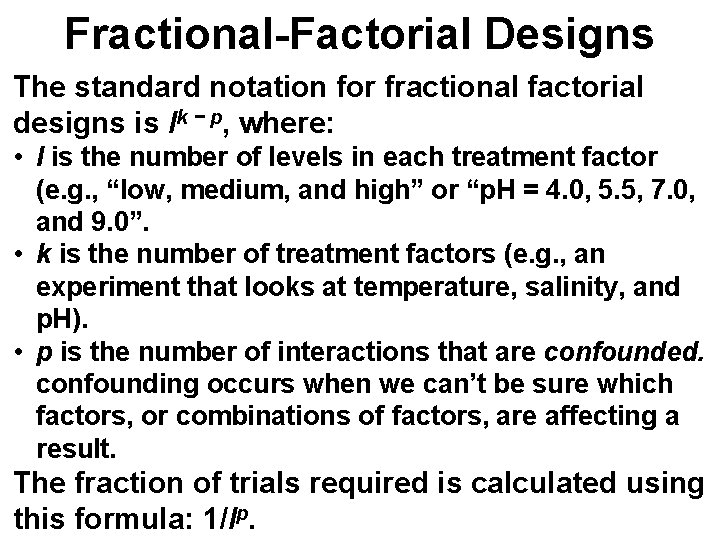
Fractional-Factorial Designs The standard notation for fractional factorial designs is lk − p, where: • l is the number of levels in each treatment factor (e. g. , “low, medium, and high” or “p. H = 4. 0, 5. 5, 7. 0, and 9. 0”. • k is the number of treatment factors (e. g. , an experiment that looks at temperature, salinity, and p. H). • p is the number of interactions that are confounded. confounding occurs when we can’t be sure which factors, or combinations of factors, are affecting a result. The fraction of trials required is calculated using this formula: 1/lp.

Fractional-Factorial Designs Consider a full factorial design that involves l = 3 levels (e. g. , low, medium, and high) in each of k = 4 treatments (A, B, C, and D). • In this case, we would assume that none of the interactions are invalid and therefore p = 0. The full factorial design would therefore require lk − p = 34 − 0 = 34 = 81 combinations. If, however, we don’t expect (or don’t care about) any interactions between two of these variables (e. g. any interactions between B and D and between either of them and A and C), then lk − p = 34 − 2 = 32 = 9 combinations. The fraction of trials required is thus 1/32 = 1/9 of the full
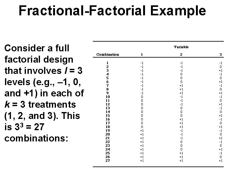
Fractional-Factorial Example Consider a full factorial design that involves l = 3 levels (e. g. , – 1, 0, and +1) in each of k = 3 treatments (1, 2, and 3). This is 33 = 27 combinations:
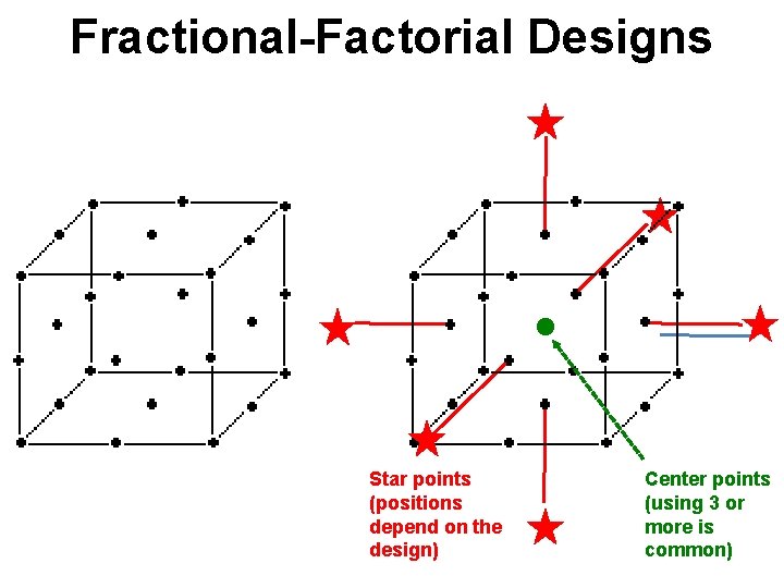
Fractional-Factorial Designs Star points (positions depend on the design) Center points (using 3 or more is common)

Fractional-Factorial Example In a central composite fractional factorial design, one creates “star points” using multiples of the original treatment levels. In the case of the goldfish experiment these are: One also needs to create 3 to 5 replicate “center points”, which are spaced through the treatment runs (which are otherwise done in random order). • There are calculators online that can assist you in determining the proper combinations and star points.
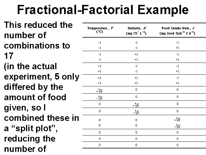
Fractional-Factorial Example This reduced the number of combinations to 17 (in the actual experiment, 5 only differed by the amount of food given, so I combined these in a “split plot”, reducing the number of

Multiple-Partial 2 R Tests • Allows examination of variables and the interactions among them. • Allows ranking of the importance of model components in making predictions. • Provides a guide for future research efforts.
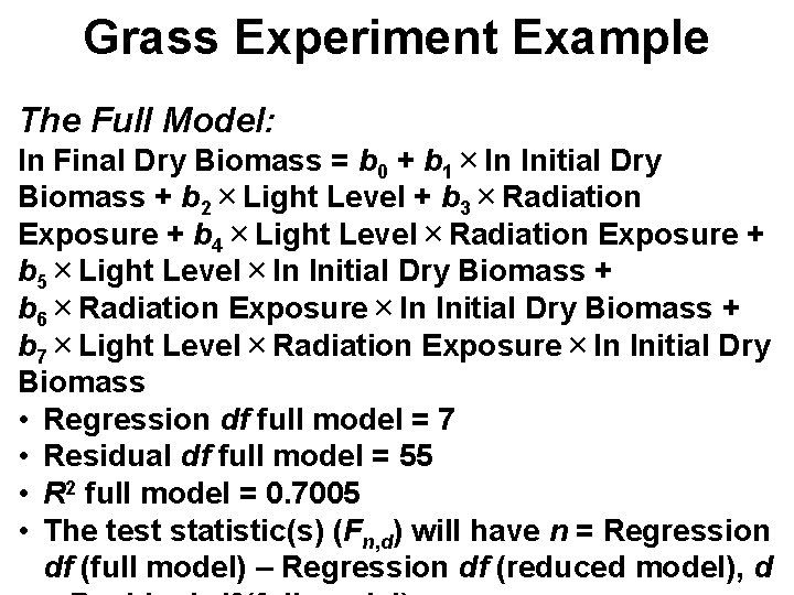
Grass Experiment Example The Full Model: ln Final Dry Biomass = b 0 + b 1×ln Initial Dry Biomass + b 2×Light Level + b 3×Radiation Exposure + b 4×Light Level×Radiation Exposure + b 5×Light Level×ln Initial Dry Biomass + b 6×Radiation Exposure×ln Initial Dry Biomass + b 7×Light Level×Radiation Exposure×ln Initial Dry Biomass • Regression df full model = 7 • Residual df full model = 55 • R 2 full model = 0. 7005 • The test statistic(s) (Fn, d) will have n = Regression df (full model) – Regression df (reduced model), d
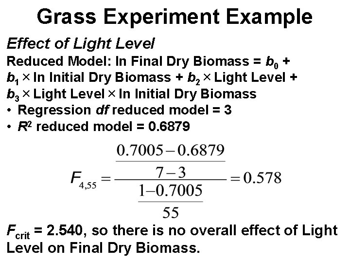
Grass Experiment Example Effect of Light Level Reduced Model: ln Final Dry Biomass = b 0 + b 1×ln Initial Dry Biomass + b 2×Light Level + b 3×Light Level×ln Initial Dry Biomass • Regression df reduced model = 3 • R 2 reduced model = 0. 6879 Fcrit = 2. 540, so there is no overall effect of Light Level on Final Dry Biomass.
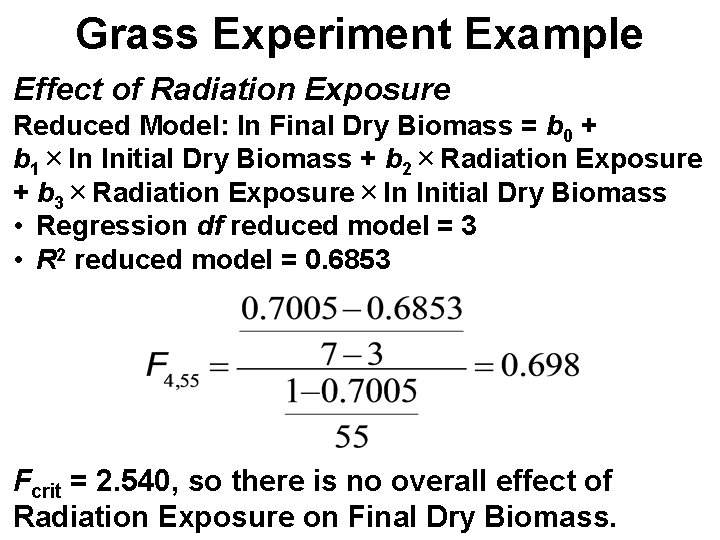
Grass Experiment Example Effect of Radiation Exposure Reduced Model: ln Final Dry Biomass = b 0 + b 1×ln Initial Dry Biomass + b 2×Radiation Exposure + b 3×Radiation Exposure×ln Initial Dry Biomass • Regression df reduced model = 3 • R 2 reduced model = 0. 6853 Fcrit = 2. 540, so there is no overall effect of Radiation Exposure on Final Dry Biomass.
Using Ranks GLM methods have a some assumptions and sensitivities to error when these are not met: • Meeting the assumption of homoscedasticity (equal variances among groups) is often particularly difficult. • Meeting the assumptions of normality is also often a challenge. In next week’s class, we will consider tests that are analogs of so-called “parametric” tests such as t-tests, tests of correlation, and GLMs, but ranks can be used in conventional
Species Diversity Measures Species Richness (S): the number of different species in a given area Shannon’s Evenness Index (E): how equal the species’ populations are numerically: • Ranges from 0 (no evenness) to 1 (perfect evenness) Shannon-Wiener Index (H): a measurement of biodiversity that incorporates both Species Richness and Species Evenness • Rarer types have a greater influence. • Ranges from 0 (no diversity) to higher values (representing more diversity).
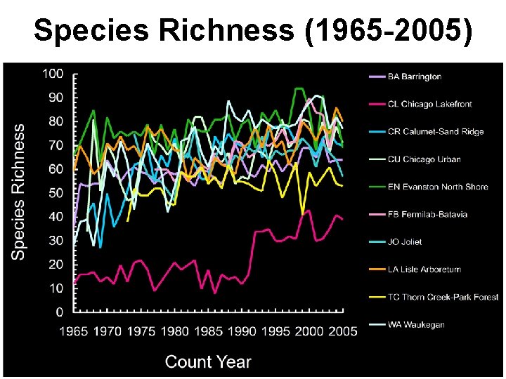
Species Richness (1965 -2005)
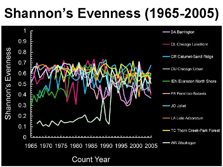
Shannon’s Evenness (1965 -2005)
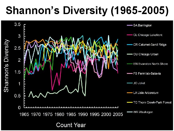
Shannon’s Diversity (1965 -2005)
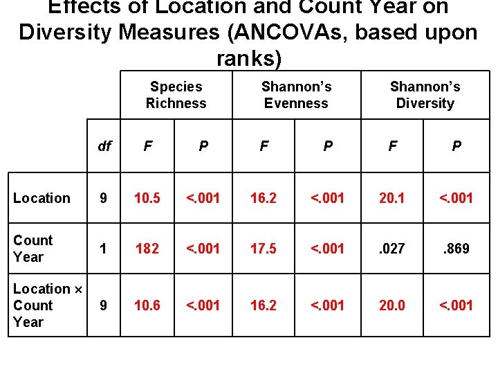
Effects of Location and Count Year on Diversity Measures (ANCOVAs, based upon ranks) Species Richness Shannon’s Evenness Shannon’s Diversity df F P F P Location 9 10. 5 <. 001 16. 2 <. 001 20. 1 <. 001 Count Year 1 182 <. 001 17. 5 <. 001 . 027 . 869 Location Count Year 9 10. 6 <. 001 16. 2 <. 001 20. 0 <. 001
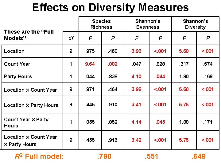
Effects on Diversity Measures Species Richness Shannon’s Evenness Shannon’s Diversity These are the “Full Models” df F P F P Location 9 . 975 . 460 3. 96 <. 001 5. 60 <. 001 Count Year 1 9. 64 . 002 . 047 . 828 . 317 . 574 Party Hours 1 . 044 . 838 4. 10 . 044 1. 90 . 169 Location Count Year 9 . 971 . 464 3. 96 <. 001 5. 60 <. 001 Location Party Hours 9 . 445 . 910 3. 41 <. 001 5. 75 <. 001 Count Year Party Hours 1 . 035 . 852 4. 14 . 043 1. 88 . 171 Location Count Year Party Hours 9 . 435 . 916 3. 42 <. 001 5. 75 <. 001 R 2 Full model: . 790 . 551 . 649
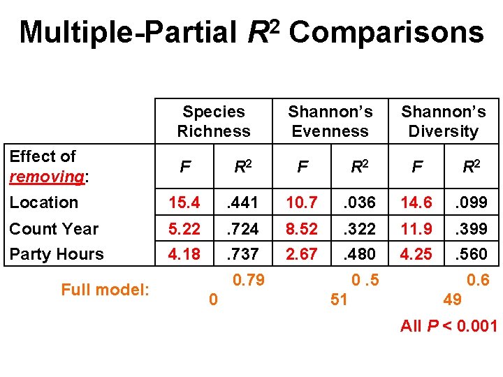
Multiple-Partial R 2 Comparisons Species Richness Effect of removing: Shannon’s Evenness Shannon’s Diversity F R 2 Location 15. 4 . 441 10. 7 . 036 14. 6 . 099 Count Year 5. 22 . 724 8. 52 . 322 11. 9 . 399 Party Hours 4. 18 . 737 2. 67 . 480 4. 25 . 560 Full model: 0. 79 0 0. 5 51 0. 6 49 All P < 0. 001
- Slides: 23