Esensing Big Earth Observation Data Handling And Analysis

E-sensing: Big Earth Observation Data Handling And Analysis On Array Databases Gilberto Câmara National Institute for Space Research (INPE), Brazil Institute for Geoinformatics, University of Münster, Germany

Be careful what you wish for…

Geoinformatics enables crucial links between nature and society Nature: Physical equations describe processes Society: Decisions on how to use Earth´s resources

mobile devices social network Mobile devices, crowdsourcing, massive Earth observation sets: new technologies, new challenges sensors everywhere ubiquitous imagery

Semantics of big data Records of interaction on human societies primary aim: communication

Semantics of big data Observations of nature primary aim: description

Semantics of big data Measurements of nature-society interaction primary aim: sustainability

Why do we need big data? Data sources: INPE, NASA. Analysis by M. Buurman

Earth Observation data is now free…and big Image source: NASA Sentinels: 3 Tb/day

What’s in an image? image: LAF/INPE “Remote sensing images describe landscape dynamics” (Câmara et al. , COSIT 2001)

Deforestation event detection: images and time series images: INPE 2010 2011

Time series analysis of land change Pasture Forest Área 1 Forest Área 2 Forest Agriculture Área 3 Vegetation index time series source: Victor Maus (INPE)

Is free data download our answer? Currently, users download one snapshot at a time How do you download a petabyte? images: INPE

What do these data have in common?

Scientific data: multidimensional arrays t y X g = f (<x, y, z> [a 1, …. an])

“Cubing” remote sensing images Landsat images ce spa Dice… time Tile squares &… Stack An Australian Geoscience Data Cube

Array databases: all data from a sensor put together in a single array t y result = analysis_function (points in space-time ) X

Sci. DB Architecture: “shared nothing” image: Paul Brown (Paradigm 4) Large data is broken into chunks Distributed server process data in paralel

Sci. DB vs. RDBMSs on storage efficiency & complex computations 16 cells 48 cells source: Paul Brown (Paradigm 4) 1. Speeds up data access in a distributed database 2. Dramatic storage efficiencies as # of dimensions & attributes grows 3. Facilitates drill-down & clustering by like groups 4. Math functions like linear algebra run directly on native storage format

An example of array algebra using MODIS data set image: NASA MODIS: 36 spectral bands, global images every 2 days

Sci. DB Architecture: “shared nothing” image: Paul Brown (Paradigm 4) Can we reproduce a Science paper? Large data is broken into chunks Distributed server process data in paralel

MOD 09 Q 1 product image: NASA 250 mts spatial resolution, 8 days temporal resolution 4800 x 4800 pixels, 3 bands (red, nir, qc) 13 years of data (since 2000)

Did Amazon forests green up during 2005 drought? (An exercise on reproducible science) July - September 2005 standardized anomalies (A) precipitation (TRMM 1998– 2006) (B) forest canopy “greenness” (MODIS EVI 2000– 2006) Published by AAAS S R Saleska et al. , Science 2007; 318: 612

Reproducing Saleska’s paper in Science with Sci. DB Array Functional Language 1. 2. 3. 4. 5. 6. Put all MODIS EVI-related bands in a single Sci. DB array Extract the subarray covering Amazonia Compute EVI for each cell in all time steps Compute EVI mean and stdev for JAS 2000 -2006 for each cell Compute EVI mean for JAS 2005 for each cell Compare EVI mean (JAS 2005) to the JAS 2000 -2006 mean

Extracting a subarray for JAS 2000 -2006 (quality filter) store(between(filter(MOD 09 Q 1_BR_2000_2013, time_id % 46 >= 23 and time_id % 46 <= 34 and quality = 4096), 48000, 38400, 0, 67199, 52799, 275), MODIS_AMZ_BQ_JAS); dimensions: col_id, row_id, time_id attributes: red, nir, quality

Calculate EVI 2 for all cells in all time steps store(apply(MODIS_AMZ_BQ_JAS, evi 2, 2. 5*((nir - red)/(nir + 2. 4*red + 1))), MODIS_AMZ_BQ_JAS_EVI 2); attributes: red, nir, quality, evi 2 image: NASA

EVI 2 mean and stdev (JAS 2000 -2006) image: U. Arizona store (aggregate (MODIS_AMZ_BQ_JAS_EVI 2, avg(evi 2) as evi 2_avg_2000_2006, stdev(evi 2) as evi 2_stdev_2000_2006, col_id, row_id), MODIS_AMZ_BQ_JAS_EVI 2_AVG_2000_2006); Attributes: evi 2_avg_2000_2006, evi 2_stdev_2000_2006

EVI 2 mean (JAS 2005) image: U. Arizona --Filters data for 2005's 3 rd quarter store(between (MODIS_AMZ_BQ_JAS_EVI 2, 48000, 38400, 253, 67199, 52799, 264), MODIS_AMZ_BQ_JAS_EVI 2_2005); --Average for 2005's 3 rd quarter store(aggregate(MODIS_AMZ_BQ_JAS_EVI 2_2005, avg(evi 2) as evi 2_avg_jas_2005, col_id, row_id), MODIS_AMZ_BQ_JAS_EVI 2_2005_AVG);

Joining two arrays (JAS 2005 and JAS 2000 -2006) image: U. Arizona store(join (MODIS_AMZ_EVI 2_BQ_JAS_AVG_2000_2006, MODIS_AMZ_EVI 2_BQ_JAS_2005_AVG), MODIS_AMZ_EVI 2_COMP); Attributes: evi 2_avg_2000_2006, evi 2_stdev_2000_2006 evi 2_avg_jas_2005

AFL: EVI anomalies (JAS 2005) store(apply (MODIS_AMZ_EVI 2_COMP, evi_anomaly, (evi 2_avg_jas_2005 - evi 2_avg_2000_2006) /evi 2_stdev_2000_2006), MODIS_AMZ_EVI 2_ANOM);

7 lines of Sci. DB commands 4, 000 MODIS tiles (92 billion cells) 4. 6 hours processing 6 months learning curve

Current GIS is map-based Big data does not fit in the “map as set of layers” model

Big data requires new conceptual views 191610 (x) 575 (t) x 7 (λ) The Space-time Data Cube concept An Australian Geoscience Data Cube

What is a geo-sensor? Field function: Position Value “Conceiving big spatiotemporal data as fields captures their nature better than the layeroriented (s, t) view”= v measure (Câmara, Egenhofer et al. , GIScience 2014) s ⋲ S - set of locations in space t ⋲ T - is the set of times. v ⋲ V - set of values

Properties of Fields value: Position Value Positions at which estimations are made Values that are estimated for each position

Three sets of (space, value) pairs + estimator: coverage set LANDSAT images of the Aral Sea images: USGS

Field: (time, space) pairs + estimator: trajectory Virgin flight VX 112 (LAX-IAD) on 26 Apr 2012: (time, space) pairs + estimator

Field: (time, value) pairs + estimator: time series Buoy in Pacific ocean near the coast of Japan (11. 03. 2011)

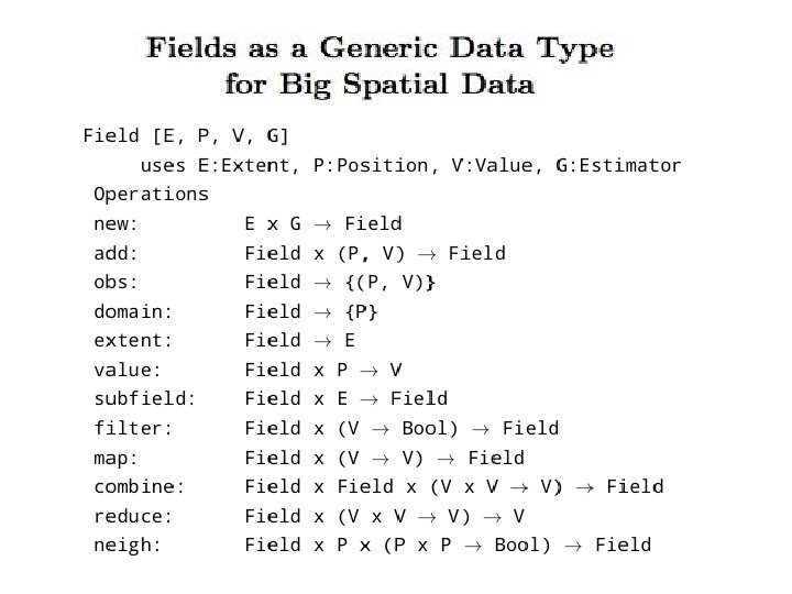
Operations on fields Field F [P: Position, V: Value, E: Extent, G: Estimator] p 2 p 3 p 1 f 1 domain(f 1)= {p 1, p 2, p 3} value (f 1, pnew) = g(f 1, pnew) pnew Domain – defines granularity Estimator provides value on all positions inside the extent

Operations on fields Three fields, same extent, different granularities, different estimators • • f 1 • • f 2 How do we express the operation f 3 = max (f 1, f 2)? • • f 3 • • •

Operations on fields Three fields, same extent, different granularities, different estimators • • f 1 • • • • f 2 • • • f 3 • • •

Map Algebra Operations Set-based algebra for operations on maps (“raster layers”) TOMLIN, D. , Geographic Information System and Cartographic Modeling, 1990. Local Focal Zonal Global

Map Algebra

Where we want to get to Remote visualization and method development Big data EO management and analysis 40 years of Earth Observation data of land change accessible for analysis and modelling.

GIS-21: Distributed data sources, unified data access Visualisation Data discovery Data access Analysis Data source Remote Analysis

Global Land Observatory: describing change in a connected world Powerful data analysis methods Array database for big scientific data Software goes where the data is! Free satellite images

Global Land Observatory: describing change in a connected world Methods for land change forestry and agriculture uses 40 years of LANDSAT + 12 years of MODIS + SENTINELs + CBERS Unique repository of knowledge and data about global land change Free satellite images