Errors on Errors Refining Statistical Analyses for Particle

“Errors on Errors” – Refining Statistical Analyses for Particle Physics Lawrence Berkeley National Lab INPA Seminar Berkeley, 21 June, 2019 Glen Cowan Physics Department Royal Holloway, University of London g. cowan@rhul. ac. uk www. pp. rhul. ac. uk/~cowan G. Cowan LBNL / 21 June 2019 / Errors on Errors 1

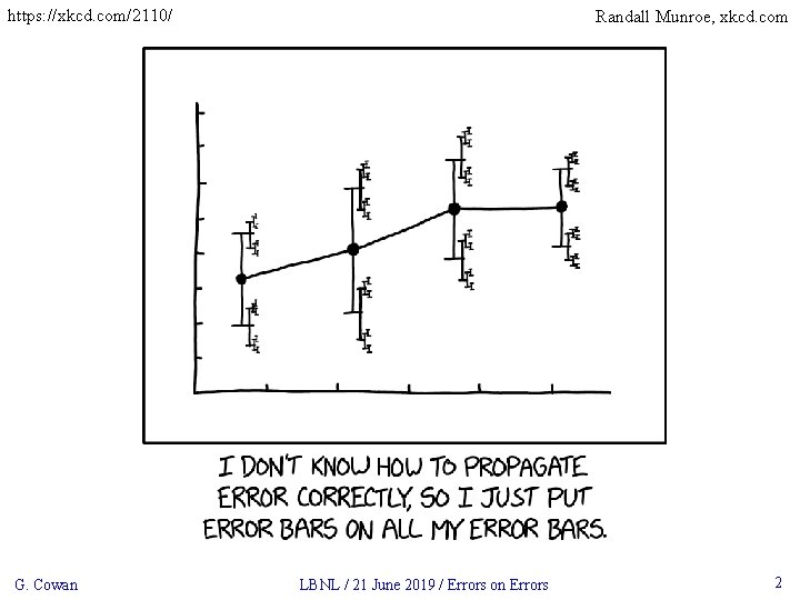
https: //xkcd. com/2110/ G. Cowan Randall Munroe, xkcd. com LBNL / 21 June 2019 / Errors on Errors 2

Outline Intro, history, motivation Using measurements with “known” systematic errors: Least Squares (BLUE) Allowing for uncertainties in the systematic errors Estimates of sys errors ~ Gamma Single-measurement model Asymptotics, Bartlett correction Curve fitting, averages Confidence intervals, goodness-of-fit, outliers Discussion and conclusions Details in: G. Cowan, Statistical Models with Uncertain Error Parameters, Eur. Phys. J. C (2019) 79: 133, ar. Xiv: 1809. 05778 G. Cowan LBNL / 21 June 2019 / Errors on Errors 3

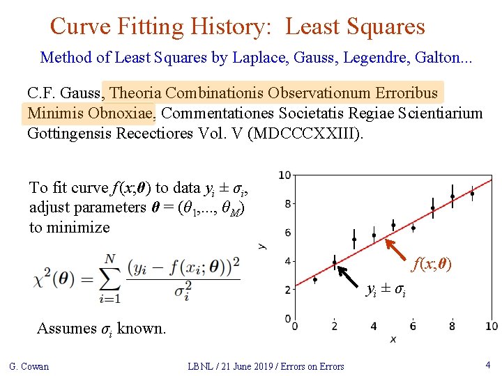
Curve Fitting History: Least Squares Method of Least Squares by Laplace, Gauss, Legendre, Galton. . . C. F. Gauss, Theoria Combinationis Observationum Erroribus Minimis Obnoxiae, Commentationes Societatis Regiae Scientiarium Gottingensis Recectiores Vol. V (MDCCCXXIII). To fit curve f (x; θ) to data yi ± σi, adjust parameters θ = (θ 1, . . . , θM) to minimize f (x; θ) y i ± σi Assumes σi known. G. Cowan LBNL / 21 June 2019 / Errors on Errors 4

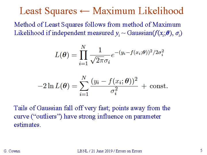
Least Squares ← Maximum Likelihood Method of Least Squares follows from method of Maximum Likelihood if independent measured yi ~ Gaussian(f (xi; θ), σi) Tails of Gaussian fall off very fast; points away from the curve (“outliers”) have strong influence on parameter estimates. G. Cowan LBNL / 21 June 2019 / Errors on Errors 5

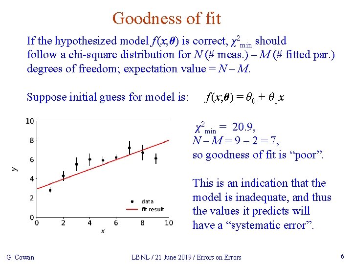
Goodness of fit If the hypothesized model f (x; θ) is correct, χ2 min should follow a chi-square distribution for N (# meas. ) – M (# fitted par. ) degrees of freedom; expectation value = N – M. Suppose initial guess for model is: f (x; θ) = θ 0 + θ 1 x χ2 min = 20. 9, N – M = 9 – 2 = 7, so goodness of fit is “poor”. This is an indication that the model is inadequate, and thus the values it predicts will have a “systematic error”. G. Cowan LBNL / 21 June 2019 / Errors on Errors 6

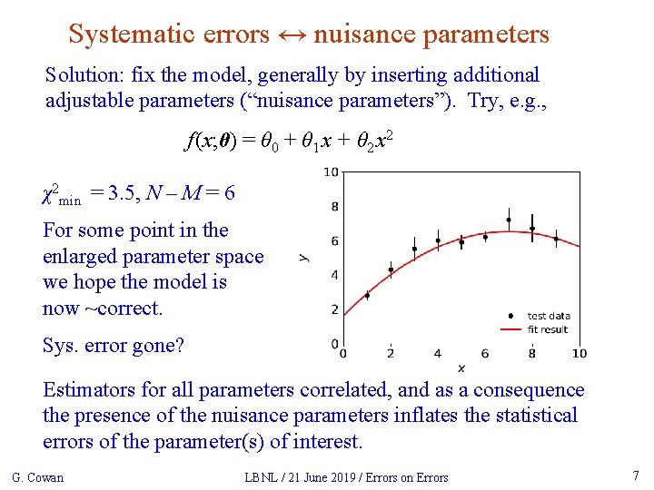
Systematic errors ↔ nuisance parameters Solution: fix the model, generally by inserting additional adjustable parameters (“nuisance parameters”). Try, e. g. , f (x; θ) = θ 0 + θ 1 x + θ 2 x 2 χ2 min = 3. 5, N – M = 6 For some point in the enlarged parameter space we hope the model is now ~correct. Sys. error gone? Estimators for all parameters correlated, and as a consequence the presence of the nuisance parameters inflates the statistical errors of the parameter(s) of interest. G. Cowan LBNL / 21 June 2019 / Errors on Errors 7

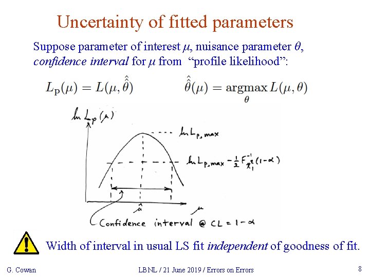
Uncertainty of fitted parameters Suppose parameter of interest μ, nuisance parameter θ, confidence interval for μ from “profile likelihood”: Width of interval in usual LS fit independent of goodness of fit. G. Cowan LBNL / 21 June 2019 / Errors on Errors 8

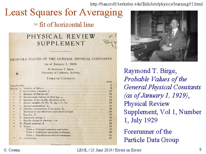
http: //bancroft. berkeley. edu/Exhibits/physics/learning 01. html Least Squares for Averaging = fit of horizontal line Raymond T. Birge, Probable Values of the General Physical Constants (as of January 1, 1929), Physical Review Supplement, Vol 1, Number 1, July 1929 Forerunner of the Particle Data Group G. Cowan LBNL / 21 June 2019 / Errors on Errors 9

Developments of LS for Averaging Much work in HEP and elsewhere on application/extension of least squares to the problem of averaging or meta-analysis, e. g. , A. C. Aitken, On Least Squares and Linear Combinations of Observations, Proc. Roy. Soc. Edinburgh 55 (1935) 42. L. Lyons, D. Gibaut and P. Clifford, How to Combine Correlated Estimates of a Single Physical Quantity, Nucl. Instr. Meth. A 270 (1988) 110. A. Valassi, Combining Correlated Measurements of Several Different Physical Quantities, Nucl. Instr. Meth. A 500 (2003) 391. R. Nisius, On the combination of correlated estimates of a physics observable, Eur. Phys. J. C 74 (2014) 3004. R. Der. Simonian and N. Laird, Meta-analysis in clinical trials, Controlled Clinical Trials 7 (1986) 177 -188. G. Cowan LBNL / 21 June 2019 / Errors on Errors 10

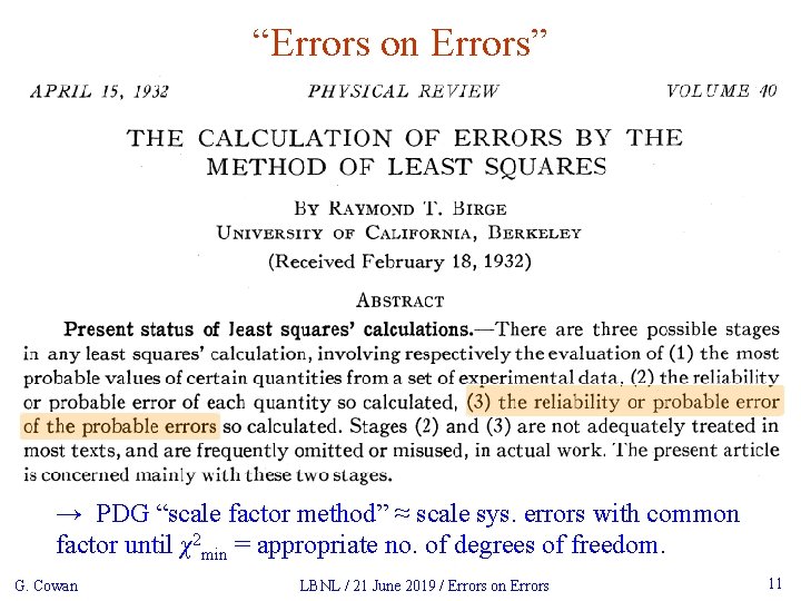
“Errors on Errors” → PDG “scale factor method” ≈ scale sys. errors with common factor until χ2 min = appropriate no. of degrees of freedom. G. Cowan LBNL / 21 June 2019 / Errors on Errors 11

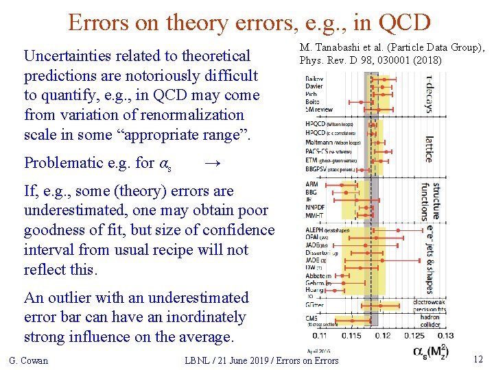
Errors on theory errors, e. g. , in QCD Uncertainties related to theoretical predictions are notoriously difficult to quantify, e. g. , in QCD may come from variation of renormalization scale in some “appropriate range”. Problematic e. g. for αs M. Tanabashi et al. (Particle Data Group), Phys. Rev. D 98, 030001 (2018) → If, e. g. , some (theory) errors are underestimated, one may obtain poor goodness of fit, but size of confidence interval from usual recipe will not reflect this. An outlier with an underestimated error bar can have an inordinately strong influence on the average. G. Cowan LBNL / 21 June 2019 / Errors on Errors 12

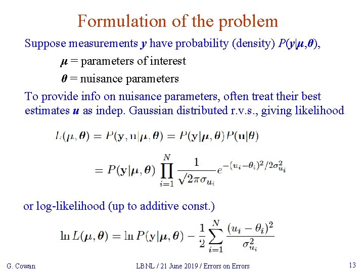
Formulation of the problem Suppose measurements y have probability (density) P(y|μ, θ), μ = parameters of interest θ = nuisance parameters To provide info on nuisance parameters, often treat their best estimates u as indep. Gaussian distributed r. v. s. , giving likelihood or log-likelihood (up to additive const. ) G. Cowan LBNL / 21 June 2019 / Errors on Errors 13

Systematic errors and their uncertainty Often the θi could represent a systematic bias and its best estimate ui in the real measurement is zero. The σu, i are the corresponding “systematic errors”. Sometimes σu, i is well known, e. g. , it is itself a statistical error known from sample size of a control measurement. Other times the ui are from an indirect measurement, Gaussian model approximate and/or the σu, i are not exactly known. Or sometimes σu, i is at best a guess that represents an uncertainty in the underlying model (“theoretical error”). In any case we can allow that the σu, i are not known in general with perfect accuracy. G. Cowan LBNL / 21 June 2019 / Errors on Errors 14

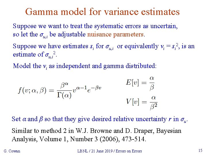
Gamma model for variance estimates Suppose we want to treat the systematic errors as uncertain, so let the σu, i be adjustable nuisance parameters. Suppose we have estimates si for σu, i or equivalently vi = si 2, is an estimate of σu, i 2. Model the vi as independent and gamma distributed: Set α and β so that they give desired relative uncertainty r in σu. Similar to method 2 in W. J. Browne and D. Draper, Bayesian Analysis, Volume 1, Number 3 (2006), 473 -514. G. Cowan LBNL / 21 June 2019 / Errors on Errors 15

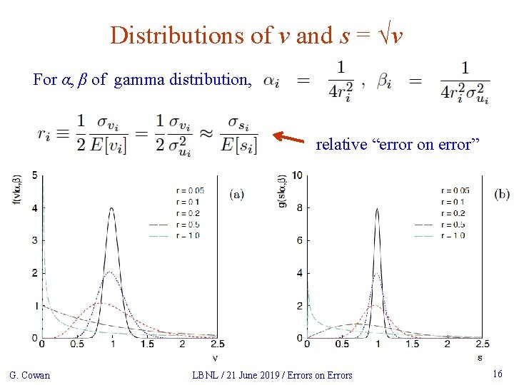
Distributions of v and s = √v For α, β of gamma distribution, relative “error on error” G. Cowan LBNL / 21 June 2019 / Errors on Errors 16

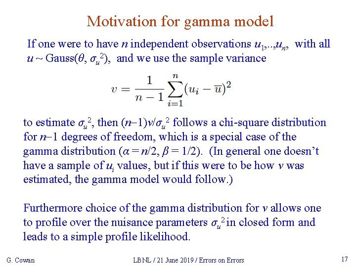
Motivation for gamma model If one were to have n independent observations u 1, . . , un, with all u ~ Gauss(θ, σu 2), and we use the sample variance to estimate σu 2, then (n-1)v/σu 2 follows a chi-square distribution for n-1 degrees of freedom, which is a special case of the gamma distribution (α = n/2, β = 1/2). (In general one doesn’t have a sample of ui values, but if this were to be how v was estimated, the gamma model would follow. ) Furthermore choice of the gamma distribution for v allows one to profile over the nuisance parameters σu 2 in closed form and leads to a simple profile likelihood. G. Cowan LBNL / 21 June 2019 / Errors on Errors 17

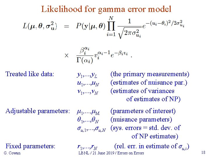
Likelihood for gamma error model Treated like data: y 1, . . . , y. L u 1, . . . , u. N v 1, . . . , v. N Adjustable parameters: μ 1, . . . , μM (parameters of interest) θ 1, . . . , θN (nuisance parameters) σu, 1, . . . , σu, N (sys. errors = std. dev. of of NP estimates) r 1, . . . , r. N (rel. err. in estimate of σu, i) Fixed parameters: G. Cowan (the primary measurements) (estimates of nuisance par. ) (estimates of variances of estimates of NP) LBNL / 21 June 2019 / Errors on Errors 18

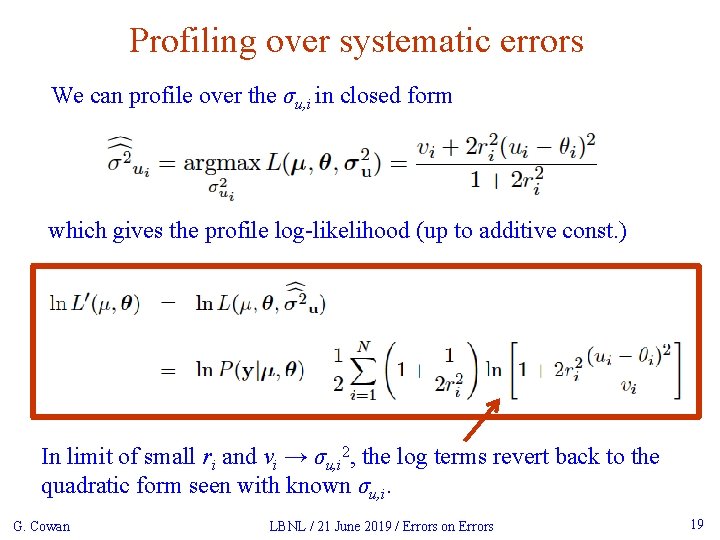
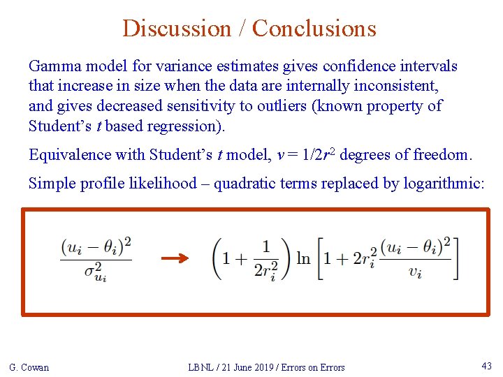
Profiling over systematic errors We can profile over the σu, i in closed form which gives the profile log-likelihood (up to additive const. ) In limit of small ri and vi → σu, i 2, the log terms revert back to the quadratic form seen with known σu, i. G. Cowan LBNL / 21 June 2019 / Errors on Errors 19

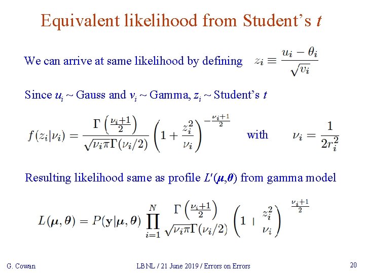
Equivalent likelihood from Student’s t We can arrive at same likelihood by defining Since ui ~ Gauss and vi ~ Gamma, zi ~ Student’s t with Resulting likelihood same as profile Lʹ(μ, θ) from gamma model G. Cowan LBNL / 21 June 2019 / Errors on Errors 20

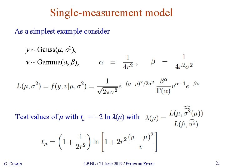
Single-measurement model As a simplest example consider y ~ Gauss(μ, σ2), v ~ Gamma(α, β), Test values of μ with tμ = -2 ln λ(μ) with G. Cowan LBNL / 21 June 2019 / Errors on Errors 21

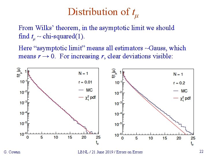
Distribution of tμ From Wilks’ theorem, in the asymptotic limit we should find tμ ~ chi-squared(1). Here “asymptotic limit” means all estimators ~Gauss, which means r → 0. For increasing r, clear deviations visible: G. Cowan LBNL / 21 June 2019 / Errors on Errors 22

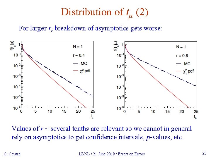
Distribution of tμ (2) For larger r, breakdown of asymptotics gets worse: Values of r ~ several tenths are relevant so we cannot in general rely on asymptotics to get confidence intervals, p-values, etc. G. Cowan LBNL / 21 June 2019 / Errors on Errors 23

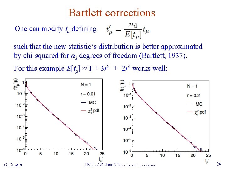
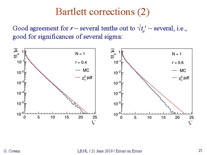
Bartlett corrections One can modify tμ defining such that the new statistic’s distribution is better approximated by chi-squared for nd degrees of freedom (Bartlett, 1937). For this example E[tμ] ≈ 1 + 3 r 2 + 2 r 4 works well: G. Cowan LBNL / 21 June 2019 / Errors on Errors 24

Bartlett corrections (2) Good agreement for r ~ several tenths out to √tμʹ ~ several, i. e. , good for significances of several sigma: G. Cowan LBNL / 21 June 2019 / Errors on Errors 25

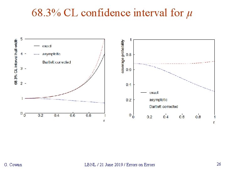
68. 3% CL confidence interval for μ G. Cowan LBNL / 21 June 2019 / Errors on Errors 26

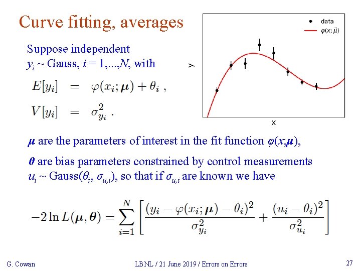
Curve fitting, averages Suppose independent yi ~ Gauss, i = 1, . . . , N, with μ are the parameters of interest in the fit function φ(x; μ), θ are bias parameters constrained by control measurements ui ~ Gauss(θi, σu, i), so that if σu, i are known we have G. Cowan LBNL / 21 June 2019 / Errors on Errors 27

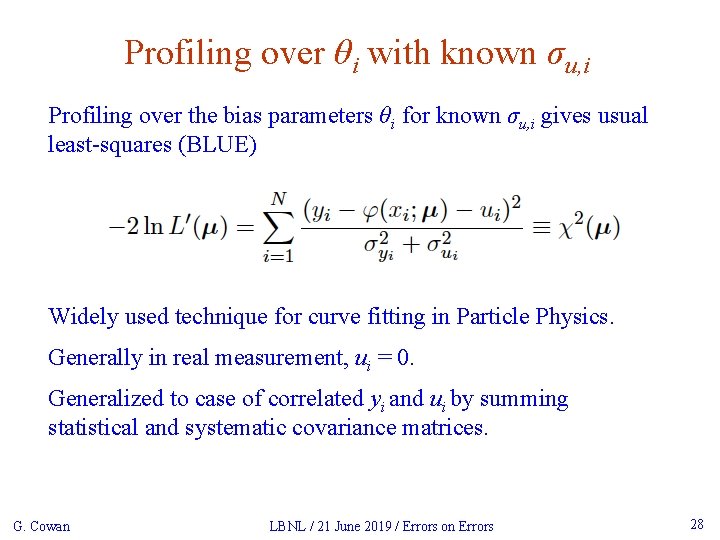
Profiling over θi with known σu, i Profiling over the bias parameters θi for known σu, i gives usual least-squares (BLUE) Widely used technique for curve fitting in Particle Physics. Generally in real measurement, ui = 0. Generalized to case of correlated yi and ui by summing statistical and systematic covariance matrices. G. Cowan LBNL / 21 June 2019 / Errors on Errors 28

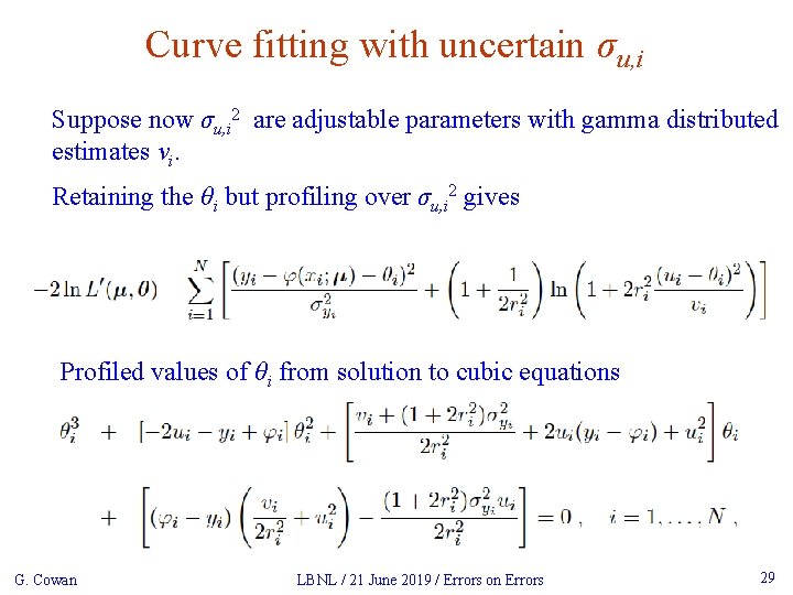
Curve fitting with uncertain σu, i Suppose now σu, i 2 are adjustable parameters with gamma distributed estimates vi. Retaining the θi but profiling over σu, i 2 gives Profiled values of θi from solution to cubic equations G. Cowan LBNL / 21 June 2019 / Errors on Errors 29

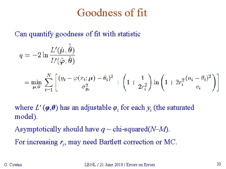
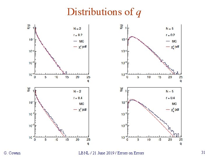
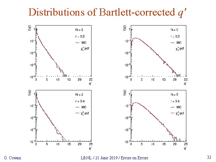
Goodness of fit Can quantify goodness of fit with statistic where Lʹ (φ, θ) has an adjustable φi for each yi (the saturated model). Asymptotically should have q ~ chi-squared(N-M). For increasing ri, may need Bartlett correction or MC. G. Cowan LBNL / 21 June 2019 / Errors on Errors 30

Distributions of q G. Cowan LBNL / 21 June 2019 / Errors on Errors 31

Distributions of Bartlett-corrected qʹ G. Cowan LBNL / 21 June 2019 / Errors on Errors 32

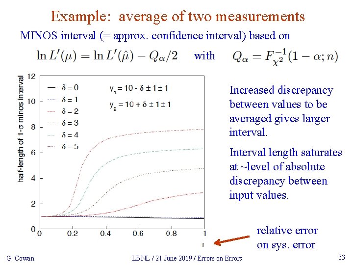
Example: average of two measurements MINOS interval (= approx. confidence interval) based on with Increased discrepancy between values to be averaged gives larger interval. Interval length saturates at ~level of absolute discrepancy between input values. relative error on sys. error G. Cowan LBNL / 21 June 2019 / Errors on Errors 33

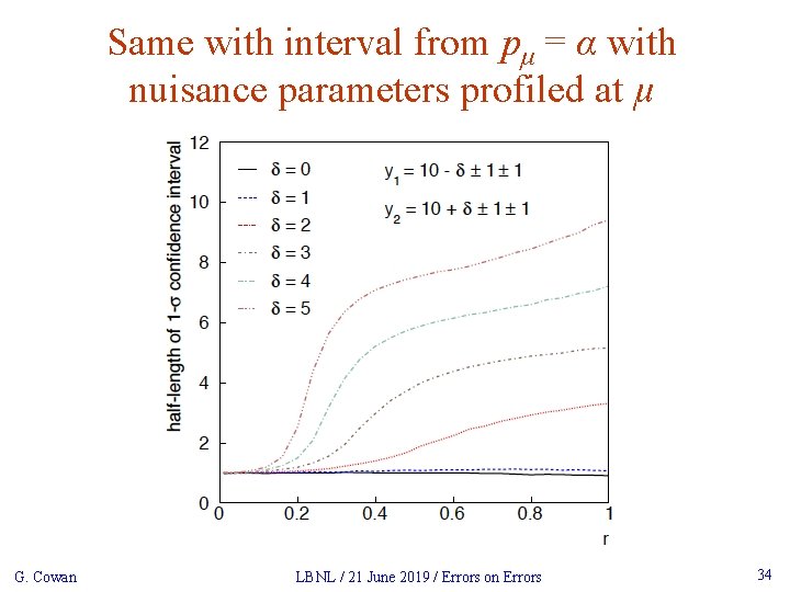
Same with interval from pμ = α with nuisance parameters profiled at μ G. Cowan LBNL / 21 June 2019 / Errors on Errors 34

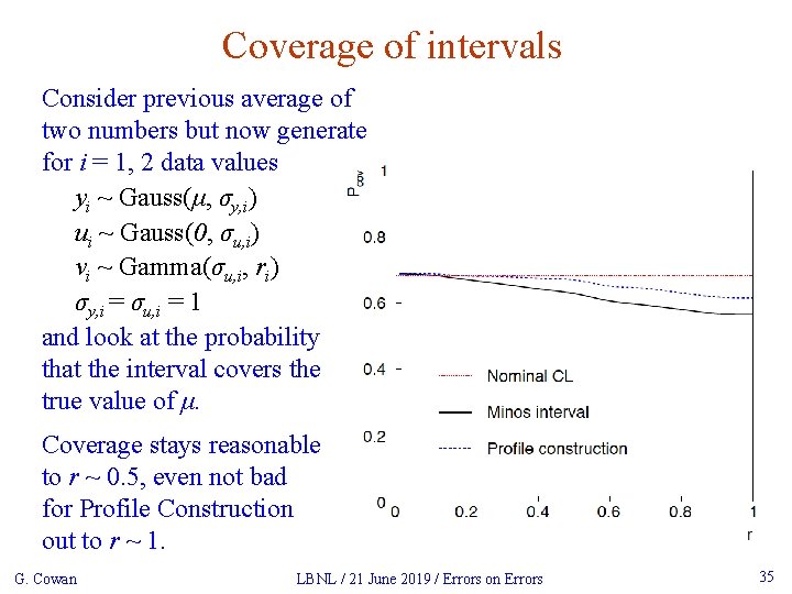
Coverage of intervals Consider previous average of two numbers but now generate for i = 1, 2 data values yi ~ Gauss(μ, σy, i) ui ~ Gauss(0, σu, i) vi ~ Gamma(σu, i, ri) σy, i = σu, i = 1 and look at the probability that the interval covers the true value of μ. Coverage stays reasonable to r ~ 0. 5, even not bad for Profile Construction out to r ~ 1. G. Cowan LBNL / 21 June 2019 / Errors on Errors 35

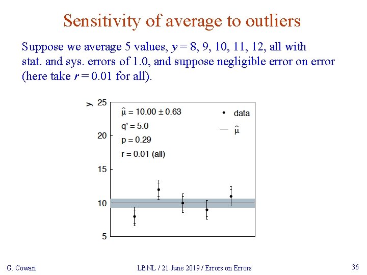
Sensitivity of average to outliers Suppose we average 5 values, y = 8, 9, 10, 11, 12, all with stat. and sys. errors of 1. 0, and suppose negligible error on error (here take r = 0. 01 for all). G. Cowan LBNL / 21 June 2019 / Errors on Errors 36

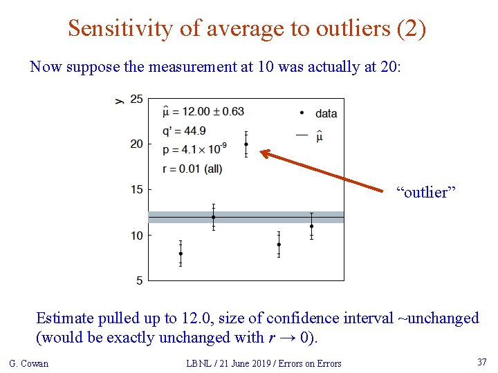
Sensitivity of average to outliers (2) Now suppose the measurement at 10 was actually at 20: “outlier” Estimate pulled up to 12. 0, size of confidence interval ~unchanged (would be exactly unchanged with r → 0). G. Cowan LBNL / 21 June 2019 / Errors on Errors 37

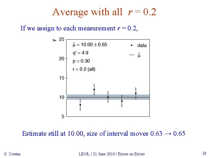
Average with all r = 0. 2 If we assign to each measurement r = 0. 2, Estimate still at 10. 00, size of interval moves 0. 63 → 0. 65 G. Cowan LBNL / 21 June 2019 / Errors on Errors 38

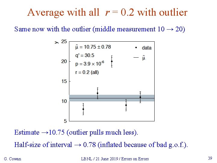
Average with all r = 0. 2 with outlier Same now with the outlier (middle measurement 10 → 20) Estimate → 10. 75 (outlier pulls much less). Half-size of interval → 0. 78 (inflated because of bad g. o. f. ). G. Cowan LBNL / 21 June 2019 / Errors on Errors 39

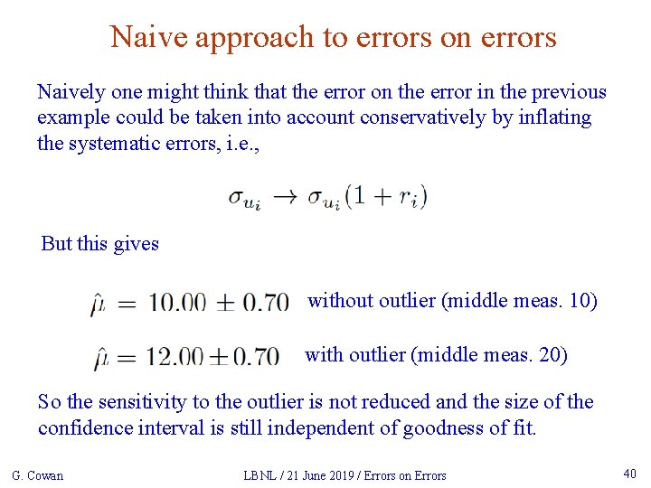
Naive approach to errors on errors Naively one might think that the error on the error in the previous example could be taken into account conservatively by inflating the systematic errors, i. e. , But this gives without outlier (middle meas. 10) with outlier (middle meas. 20) So the sensitivity to the outlier is not reduced and the size of the confidence interval is still independent of goodness of fit. G. Cowan LBNL / 21 June 2019 / Errors on Errors 40

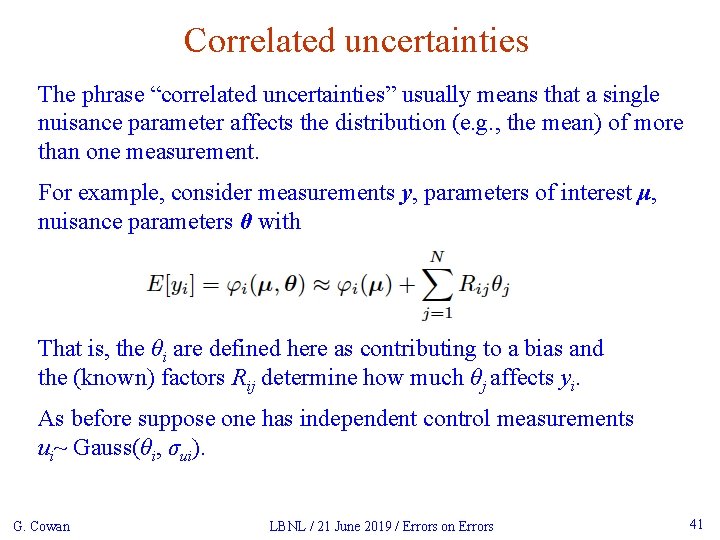
Correlated uncertainties The phrase “correlated uncertainties” usually means that a single nuisance parameter affects the distribution (e. g. , the mean) of more than one measurement. For example, consider measurements y, parameters of interest μ, nuisance parameters θ with That is, the θi are defined here as contributing to a bias and the (known) factors Rij determine how much θj affects yi. As before suppose one has independent control measurements ui~ Gauss(θi, σui). G. Cowan LBNL / 21 June 2019 / Errors on Errors 41

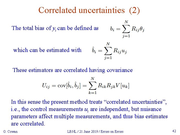
Correlated uncertainties (2) The total bias of yi can be defined as which can be estimated with These estimators are correlated having covariance In this sense the present method treats “correlated uncertainties”, i. e. , the control measurements ui are independent, but nuisance parameters affect multiple measurements, and thus bias estimates are correlated. G. Cowan LBNL / 21 June 2019 / Errors on Errors 42

Discussion / Conclusions Gamma model for variance estimates gives confidence intervals that increase in size when the data are internally inconsistent, and gives decreased sensitivity to outliers (known property of Student’s t based regression). Equivalence with Student’s t model, ν = 1/2 r 2 degrees of freedom. Simple profile likelihood – quadratic terms replaced by logarithmic: G. Cowan LBNL / 21 June 2019 / Errors on Errors 43

Discussion / Conclusions (2) Asymptotics can break for increased error-on-error, may need Bartlett correction or MC. Method assumes that meaningful ri values can be assigned and is valuable when systematic errors are not well known but enough “expert opinion” is available to do so. Alternatively one could try to fit a global r to all systematic errors, analogous to PDG scale factor method or meta-analysis à la Der. Simonian and Laird. (→ future work). Could also use e. g. as “stress test” – crank up the ri values until significance of result degrades and ask if you really trust the assigned systematic errors at that level. Decisions on new facilities require one to know how accurately important parameters have and will be measured; it’s important to get this right. G. Cowan LBNL / 21 June 2019 / Errors on Errors 44

Extra slides G. Cowan LBNL / 21 June 2019 / Errors on Errors 45

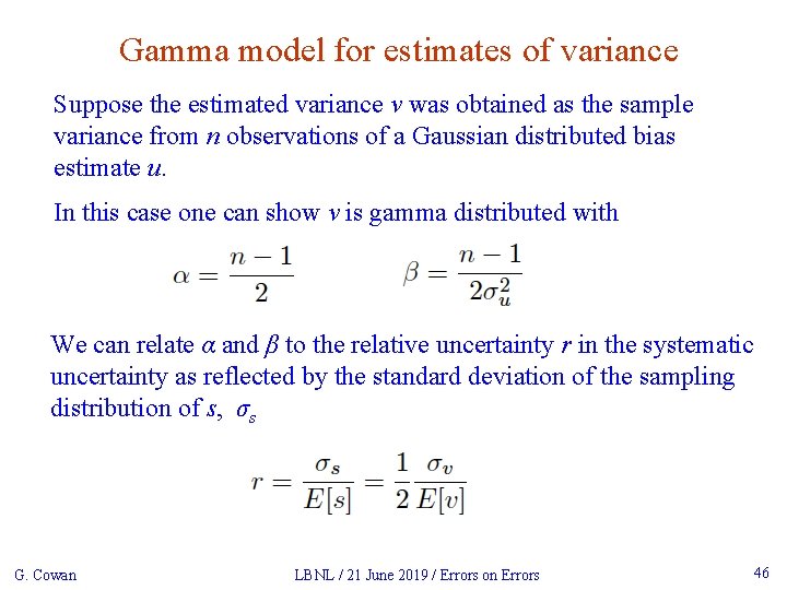
Gamma model for estimates of variance Suppose the estimated variance v was obtained as the sample variance from n observations of a Gaussian distributed bias estimate u. In this case one can show v is gamma distributed with We can relate α and β to the relative uncertainty r in the systematic uncertainty as reflected by the standard deviation of the sampling distribution of s, σs G. Cowan LBNL / 21 June 2019 / Errors on Errors 46

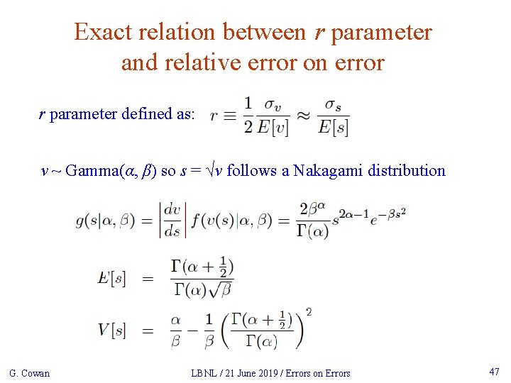
Exact relation between r parameter and relative error on error r parameter defined as: v ~ Gamma(α, β) so s = √v follows a Nakagami distribution G. Cowan LBNL / 21 June 2019 / Errors on Errors 47

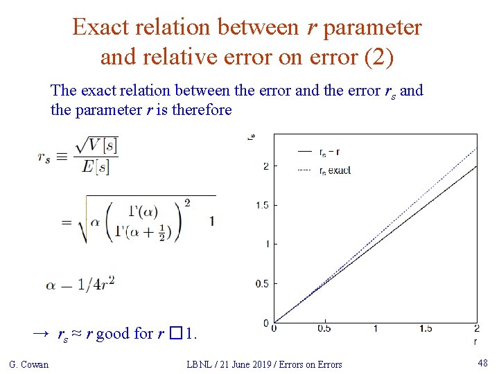
Exact relation between r parameter and relative error on error (2) The exact relation between the error and the error rs and the parameter r is therefore → rs ≈ r good for r � 1. G. Cowan LBNL / 21 June 2019 / Errors on Errors 48

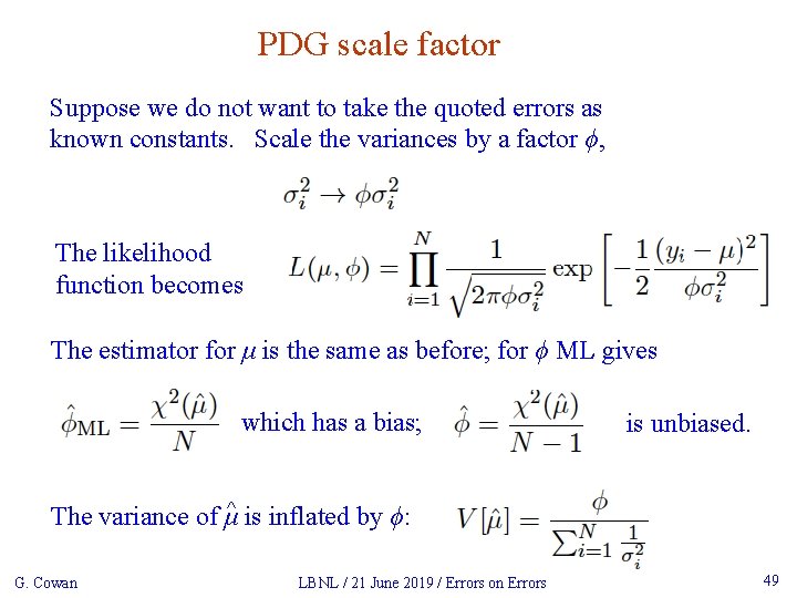
PDG scale factor Suppose we do not want to take the quoted errors as known constants. Scale the variances by a factor ϕ, The likelihood function becomes The estimator for μ is the same as before; for ϕ ML gives which has a bias; is unbiased. The variance of μ^ is inflated by ϕ: G. Cowan LBNL / 21 June 2019 / Errors on Errors 49

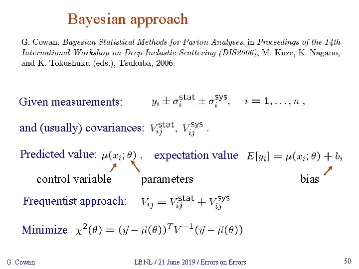
Bayesian approach Given measurements: and (usually) covariances: Predicted value: control variable expectation value parameters bias Frequentist approach: Minimize G. Cowan LBNL / 21 June 2019 / Errors on Errors 50

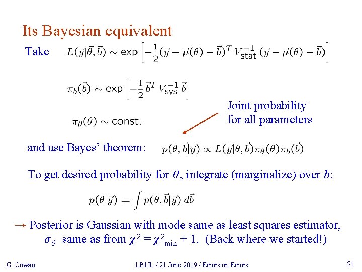
Its Bayesian equivalent Take Joint probability for all parameters and use Bayes’ theorem: To get desired probability for θ , integrate (marginalize) over b: → Posterior is Gaussian with mode same as least squares estimator, σ θ same as from χ 2 = χ 2 min + 1. (Back where we started!) G. Cowan LBNL / 21 June 2019 / Errors on Errors 51

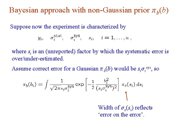
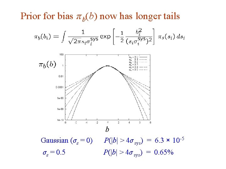
Bayesian approach with non-Gaussian prior π b(b) Suppose now the experiment is characterized by where si is an (unreported) factor by which the systematic error is over/under-estimated. Assume correct error for a Gaussian π b(b) would be siσ isys, so Width of σ s(si) reflects ‘error on the error’.

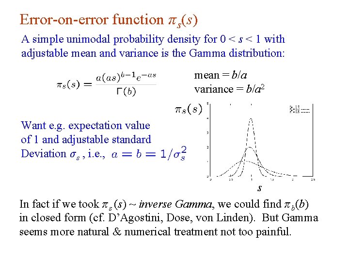
Error-on-error function π s(s) A simple unimodal probability density for 0 < s < 1 with adjustable mean and variance is the Gamma distribution: mean = b/a variance = b/a 2 Want e. g. expectation value of 1 and adjustable standard Deviation σ s , i. e. , s In fact if we took π s (s) ~ inverse Gamma, we could find π b(b) in closed form (cf. D’Agostini, Dose, von Linden). But Gamma seems more natural & numerical treatment not too painful.

Prior for bias π b(b) now has longer tails Gaussian (σs = 0) b P(|b| > 4σ sys) = 6. 3 × 10 -5 σs = 0. 5 P(|b| > 4σ sys) = 0. 65%

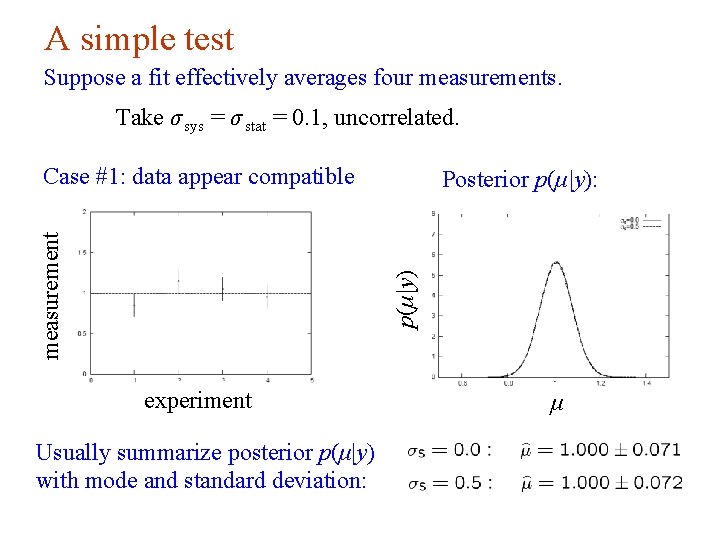
A simple test Suppose a fit effectively averages four measurements. Take σ sys = σ stat = 0. 1, uncorrelated. Posterior p(μ|y): p(μ|y) measurement Case #1: data appear compatible experiment Usually summarize posterior p(μ|y) with mode and standard deviation: μ

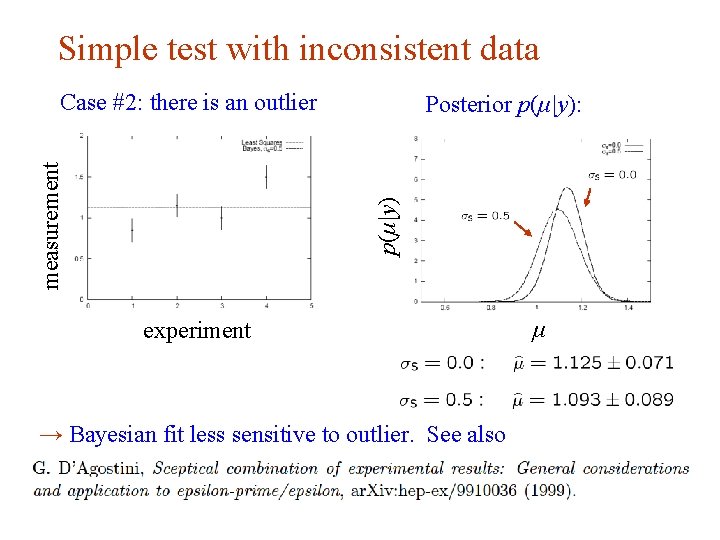
Simple test with inconsistent data Posterior p(μ|y): p(μ|y) measurement Case #2: there is an outlier experiment → Bayesian fit less sensitive to outlier. See also μ

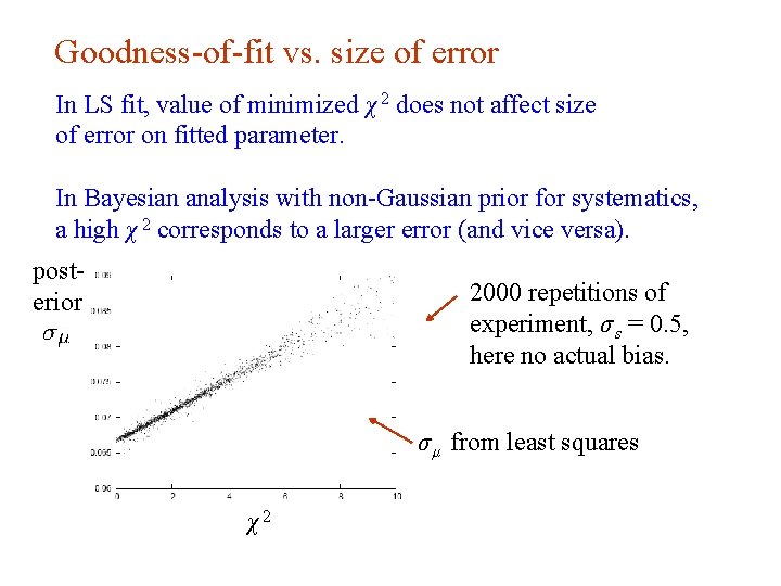
Goodness-of-fit vs. size of error In LS fit, value of minimized χ 2 does not affect size of error on fitted parameter. In Bayesian analysis with non-Gaussian prior for systematics, a high χ 2 corresponds to a larger error (and vice versa). posterior 2000 repetitions of experiment, σ s = 0. 5, here no actual bias. σ μ from least squares χ2