Error Control Coding And Data Link Control UNIT

Error Control Coding And Data Link Control UNIT IV

Error Control Coding And Data Link Control � Error Detection and Correction: Introduction, Error Detection, Error Correction � Linear Block Codes: hamming code, Hamming Distance, parity check code � Cyclic Codes: CRC (Polynomials), Advantages Of Cyclic Codes, Other Cyclic Codes As Examples: CHECKSUM: One's Complement, Internet Checksum � Framing: fixed-size framing, variable size framing. � Flow control: flow control protocols. � Noiseless channels: simplest protocol, stop-and-wait protocol. � Noisy channels: stop-and-wait automatic repeat request, goback-n automatic repeat request, Selective repeat automatic repeat request, piggybacking

Error Detection and Correction

Introduction �Networks must be able to transfer data from one device to another with complete accuracy. � Data can be corrupted during transmission. � For reliable communication, errors must be detected and corrected. � Error detection and correction are implemented either at the data link layer or the transport layer of the OSI model. �Some applications require that errors be detected and corrected e. g. text file. �While some application can tolerate errors to some extent e. g. . Audio, video

Types of Errors

Types of Errors � Single Bit Error: �In a single-bit error, only one bit in the data unit has changed from 0 to 1 or from 1 to 0.

�Burst Error: �A burst error means that 2 or more bits in the data unit have changed.

Error detection: Redundancy �Error detection means to decide whether the received data is correct or not without having a copy of the original message. �Error detection uses the concept of redundancy, which means adding extra bits for detecting errors at the destination. �To detect or correct errors, we need to send extra (redundant) bits with data. �These redundant bits are added by the sender and removed by the receiver.

The Structure of Encoder and Decoder

Four types of redundancy checks are used in data communications

Vertical Redundancy Check VRC

Performance âIt can detect single bit error âIt can detect burst errors only if the total number of errors is odd.

Longitudinal Redundancy Check LRC

Performance âLCR increases the likelihood of detecting burst errors. âIf two bits in one data units are damaged and two bits in exactly the same positions in another data unit are also damaged, the LRC checker will not detect an error.

VRC and LRC

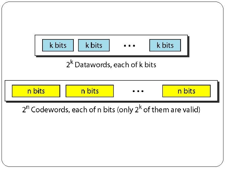
Block Coding � In block coding, we divide our message into blocks, each of k bits, called datawords. � We add r redundant bits to each block to make the length n = k + r. � The resulting n-bit blocks are called codewords. �k = dataword size �r = redundant bits �n = codeword block size �n = k + r �Since n>k so 2 n is greater than 2 k i. e. no of possible codewords is always greater than no. of possible datawords.

Error Detection �An error-detecting code can detect only the types of errors for which it is designed; other types of errors may remain undetected.

Error Correction �Error Correction is difficult than detection.

Hamming Code �Hamming codes are a family of linear error- correcting codes. �It is a set of error-correction codes that can be used to detect and correct bit errors that can occur when computer data is moved or stored.

Hamming Distance � It is central concept behind err correction. � The Hamming distance between two words is the number of differences between corresponding bits and is shown as d(x, y) � The Hamming distance can be easily found by applying XOR operation.

� Let us find the Hamming distance between two pairs of words. 1. The Hamming distance d(000, 011) is 2 because 2. The Hamming distance d(10101, 11110) is 3 because

�The minimum Hamming distance (dmin ) is the smallest Hamming distance between all possible pairs in a set of words.

Find the minimum Hamming distance of the coding scheme. Solution We first find all Hamming distances. The dmin in this case is 2.

Find the minimum Hamming distance of the coding scheme. Solution We first find all the Hamming distances. The dmin in this case is 3.

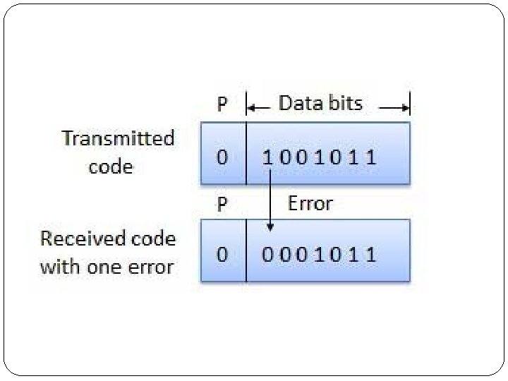
Parity Check Code �The simple parity-check code is the most familiar error-detecting code. �In this code, a k-bit data word is changed to an nbit code word where n = k + 1. �The extra bit, called the parity bit, is selected to make the total number of 1 s in the code word even. �Although some implementations specify an odd number of 1 s.

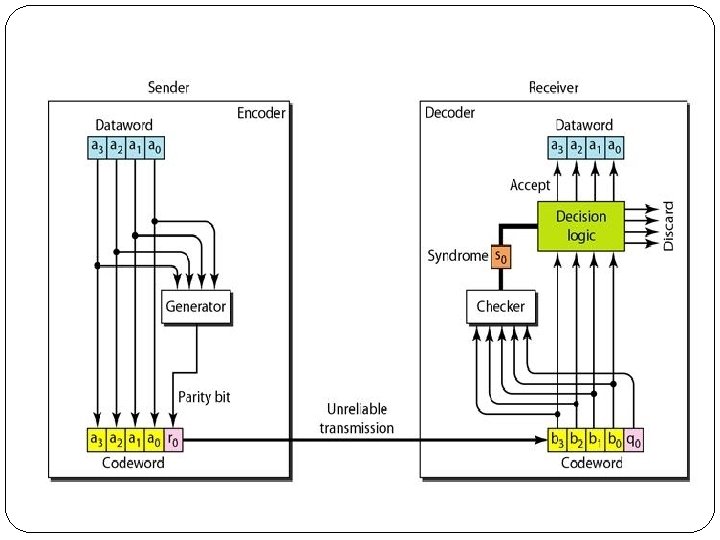
Simple Parity Check Code

�The encoder uses a generator that takes a copy of a 4 -bit data word (a 0, a 1, a 2 and a 3) and generates a parity bit r 0. �The data word bits and the parity bit create the 5 bit code word. �The parity bit that is added makes the number of 1 s in the code word even. �The result is the parity bit. �The sender sends the code word which may be corrupted during transmission. �The receiver receives a 5 -bit word.

�The checker at the receiver does the same thing as the generator in the sender with one exception: The addition is done over all 5 bits. �The result, which is called the syndrome, is just 1 bit. �The syndrome is 0 when the number of 1 s in the received code word is even; otherwise, it is 1. �The syndrome is passed to the decision logic analyzer. �If the syndrome is 0, there is no error in the received code word, the data portion of the received code word is accepted as the data

Cyclic Codes � Cyclic codes are special linear block codes with one extra property. � In a cyclic code, if a codeword is cyclically shifted (rotated), the result is another codeword.

A polynomial to represent a binary word �Polynomial can be used to represent and analyze cyclic codes. �Bits can be shown as polynomial , where power of terms x, shows position of the bit, and coefficient shows the value of bit.

Cyclic Redundancy Codes (CRC) �Parity methods detects only odd number of errors. �To overcome this weakness polynomial codes error detection method is used. �It involves generating check bits in the form of a Cyclic Redundancy Codes (CRC)

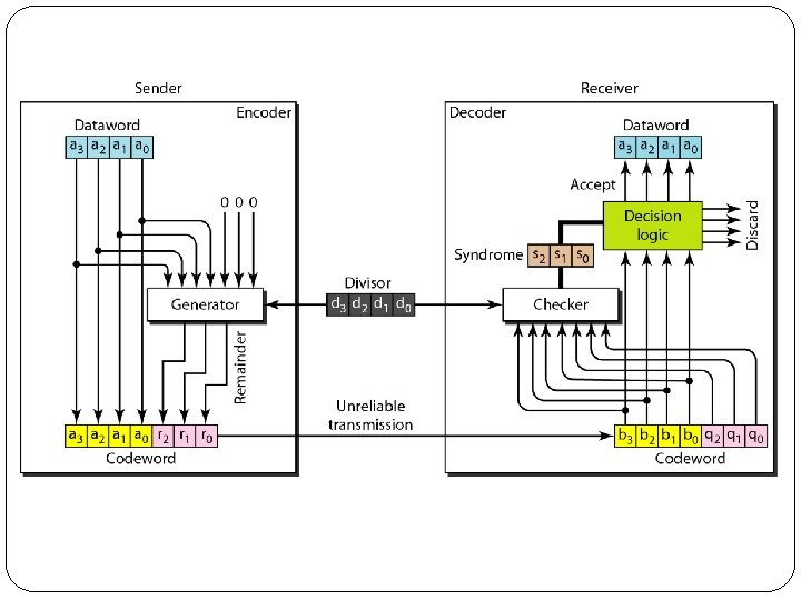
A CRC code with C(7, 4)

�Here 4 bit dataword( k=4) is appended by three 0’s ( r=3). �The size of the dataword is augmented by adding n-k (3 here) 0 s to the right hand side of the word. �It uses divisor of n-k+1 bits ( 7 -4+1=4 ), which divides the 7 bit dataword. �Quotient is discarded and remainder is appended to original 4 bit dataword to form a codeword and sent to Receiver. �At Receiver, it divides received code by same divisor , if remainder is all 0’s , the codeword is accepted, else discarded.

�The divisor in a cyclic code is normally called the generator polynomial or simply the generator g(x). �f(x): Polynomial with binary coefficient �d(x): Dataword �c(x): Codeword �e(x): Error �s(x): Syndrome �In a cyclic code, �If s(x) ≠ 0, one or more bits is corrupted. �If s(x) = 0, either a. No bit is corrupted. Or b. Some bits are corrupted, but the decoder failed to detect them.

Division in CRC encoder

Division in the CRC decoder for two cases

Advantages of Cyclic Codes �Ease of implementation �Executes faster when implemented in hardware �It detects: single bit error, odd no. of errors and burst errors

Checksum � The checksum is used in the Internet by several protocols although not at the data link layer.

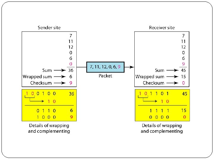
Suppose our data is a list of five 4 -bit numbers that we want to send to a destination. In addition to sending these numbers, we send the sum of the numbers. For example, if the set of numbers is (7, 11, 12, 0, 6), we send (7, 11, 12, 0, 6, 36), where 36 is the sum of the original numbers. The receiver adds the five numbers and compares the result with the sum. If the two are the same, the receiver assumes no error, accepts the five numbers, and discards the sum. Otherwise, there is an error somewhere and the data are not accepted.

We can make the job of the receiver easier if we send the negative (complement) of the sum, called the checksum. In this case, we send (7, 11, 12, 0, 6, − 36). The receiver can add all the numbers received (including the checksum). If the result is 0, it assumes no error; otherwise, there is an error.

How can we represent the number 21 in one’s complement arithmetic using only four bits? Solution The number 21 in binary is 10101 (it needs five bits). We can wrap the leftmost bit and add it to the four rightmost bits. We have (0101 + 1) = 0110 or 6.

How can we represent the number − 6 in one’s complement arithmetic using only four bits? Solution In one’s complement arithmetic, the negative or complement of a number is found by inverting all bits. Positive 6 is 0110; negative 6 is 1001. If we consider only unsigned numbers, this is 9. In other words, the complement of 6 is 9.

Figure shows the process at the sender and at the receiver. The sender initializes the checksum to 0 and adds all data items and the checksum (the checksum is considered as one data item and is shown in color). The result is 36. However, 36 cannot be expressed in 4 bits. The extra two bits are wrapped and added with the sum to create the wrapped sum value 6. In the figure, we have shown the details in binary. The sum is then complemented, resulting in the checksum value 9 (15 − 6 = 9). The sender now sends six data items to the receiver including the checksum 9.

The receiver follows the same procedure as the sender. It adds all data items (including the checksum); the result is 45. The sum is wrapped and becomes 15. The wrapped sum is complemented and becomes 0. Since the value of the checksum is 0, this means that the data is not corrupted. The receiver drops the checksum and keeps the other data items. If the checksum is not zero, the entire packet is dropped.

Internet Checksum � The Internet has been using a 16 -bit checksum and uses following steps: � Sender Site: 1. The message is divided into 16 -bit words. 2. The value of the checksum word is set to 0. 3. All words including the checksum are added using one’s complement addition. 4. The sum is complemented and becomes the checksum. 5. The checksum is sent with the data.

�Receiver Site: 1. The message (including checksum) is divided into 16 bit words. 2. All words are added using one’s complement addition. 3. The sum is complemented and becomes the new checksum. 4. If the value of checksum is 0, the message is accepted; otherwise, it is rejected.

Framing

� The Data Link Layer is the second layer in the OSI model, above the Physical Layer, which ensures that the error free data is transferred between the adjacent nodes in the network. � It breaks the datagrams passed down by above layers and convert them into frames ready for transfer. � This is called Framing. � It provides two main functionalities: �Reliable data transfer service between two peer network layers �Flow Control mechanism which regulates the flow of frames such that data congestion is not there at slow receivers due to fast senders. � The data link layer needs to pack bits into frames, so that each frame is distinguishable from another.

Framing Types: Fixed-Size Framing �In fixed-size framing, there is no need for defining the boundaries of the frames; the size itself can be used as a delimiter. �An example of this type of framing is the ATM wide-area network, which uses frames of fixed size called cells.

Framing Types: Variable-Size Framing �In variable-size framing, we need a way to define the end of the frame and the beginning of the next. Historically, two approaches were used for this purpose: �A character-oriented approach �A bit-oriented approach

Flow and Error Control � The most important responsibilities of the data link layer are flow control and error control. � Collectively, these functions are known as data link control. � Flow control refers to a set of procedures used to restrict the amount of data that the sender can send before waiting for acknowledgment. �Error control in the data link layer is based on automatic repeat request, which is the retransmission of data.

Protocols � The protocols are normally implemented in software by using one of the common programming languages.

Noiseless Channels �An ideal channel in which no frames are lost, duplicated, or corrupted.

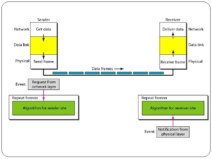
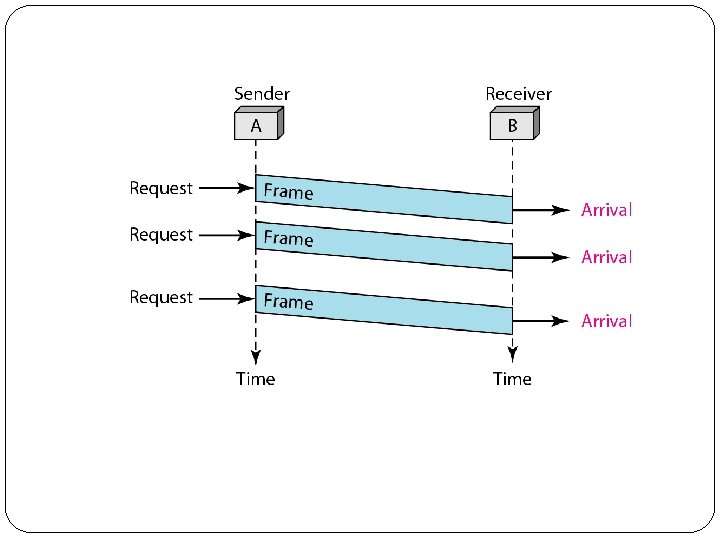
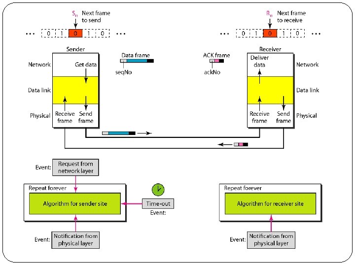
1. Simplest Protocol �This is one with no flow and no error control. �No flow control since Receiver can immediately handle (accept) any frame it receives i. e. processes it within no time (removes header and trailer) and passes to network layer. �The DLL at Sender cant send any data until it receives data it from its upper network layer. �The DLL at Receiver cant send any data until it receives data it from its lower physical layer. �So we need to introduce idea of events.

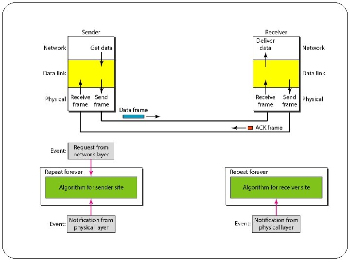
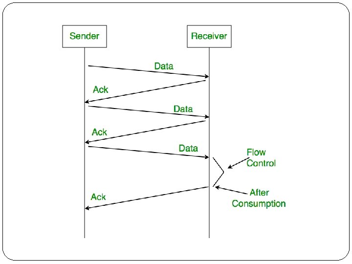
2. Stop-and-wait Protocol �Faster Sender –Slower Receiver, Receiver has limited Buffer �The sender sends one frame, stops until it receives confirmation from the receiver and then sends the next frame

Noiseless channels �In practice noiseless channels are nonexistent. �Three protocols in this section that use error control. �Stop-and-Wait Automatic Repeat Request �Go-Back-N Automatic Repeat Request �Selective Repeat Automatic Repeat Request

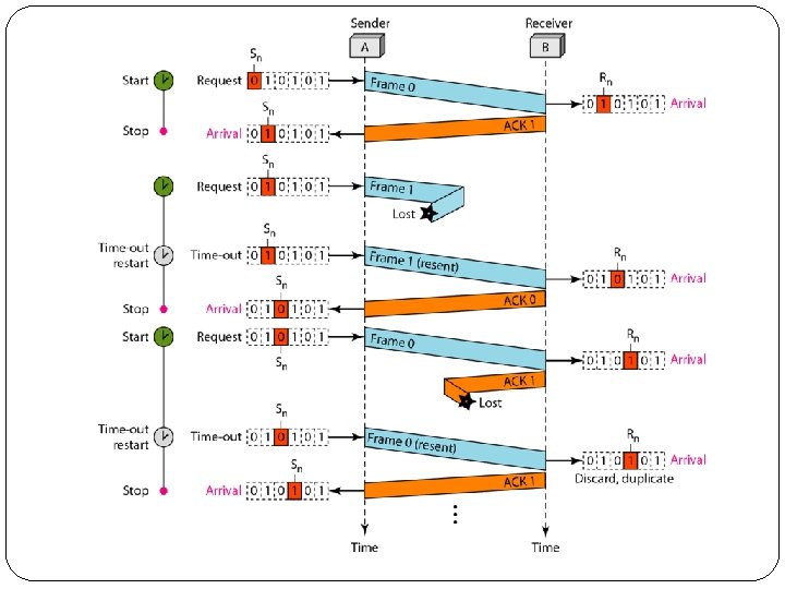
1. Stop-and-Wait Automatic Repeat Request �It adds a simple error control mechanism to Stop- and-Wait �Error correction in Stop-and-Wait ARQ is done by keeping a copy of the sent frame and retransmitting of the frame when the timer expires.

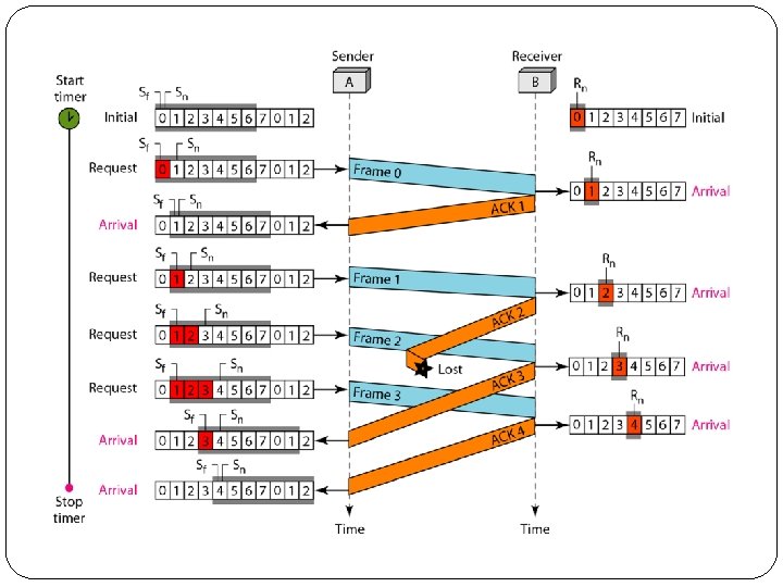
2. Go-Back-N Automatic Repeat Request �To improve the efficiency of transmission (filling the pipe), multiple frames must be in transition while waiting for acknowledgment. �In Go-Back-N Automatic Repeat Request, we can send several frames before receiving acknowledgments; we keep a copy of these frames until the acknowledgments arrive.

� Sequence Numbers �Frames from a sending station are numbered sequentially. �If the header of the frame allows m bits for the sequence number, the sequence numbers range from 0 to 2 m- 1. �For example, if m is 4, the only sequence numbers are 0 through 15 inclusive. �However, we can repeat the sequence. So the sequence numbers are 0, 1, 2, 3, 4, 5, 6, 7, 8, 9, 10, 11, 12, 13, 14, 15, 0, 1, 2, 3, 4, 5, 6, 7, 8, 9, 10, 11, . . . �In other words, the sequence numbers are modulo-2 m.

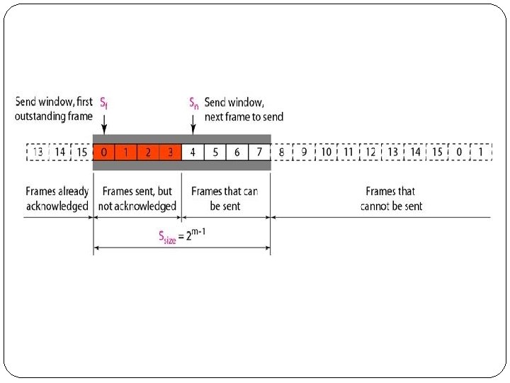
�Sliding Window �In this protocol (and the next), the sliding window is an abstract concept that defines the range of sequence numbers that is the concern of the sender and receiver. �In other words, the sender and receiver need to deal with only part of the possible sequence numbers. �The range which is the concern of the sender is called the send sliding window; the range that is the concern of the receiver is called the receiver sliding window. �The send window is an imaginary box covering the sequence numbers of the data frames which can be in transit. �In each window position, some of these sequence numbers define the frames that have been sent; others define those that can be sent.

Send window for Go-Back-N ARQ

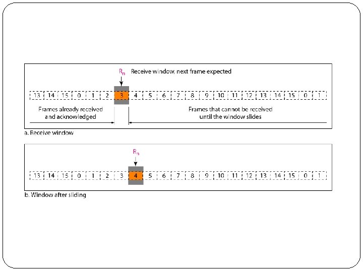
�The maximum size of the window is 2 m – 1. �The size can be fixed and set to the maximum value. �The following figure shows a sliding window of size 15 (m =4). �The receive window makes sure that the correct data frames are received and that the correct acknowledgments are sent. �The size of the receive window is always I. �The receiver is always looking for the arrival of a specific frame. �Any frame arriving out of order is discarded and needs to be resent.

Design of Go-Back-N ARQ

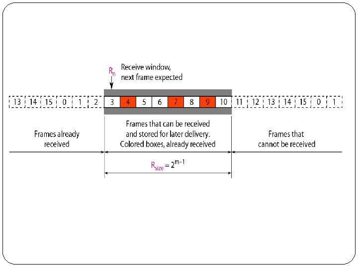
3. Selective Repeat Automatic Repeat Request � Go-Back-N ARQ simplifies the process at the receiver site. � The receiver keeps track of only one variable, and there is no need to buffer out-of-order frames; they are simply discarded. � However, this protocol is very inefficient for a noisy link. � The Selective Repeat Protocol also uses two windows: a send window and a receive window. � However, there are differences between the windows in this protocol and the ones in Go-Back-N. � First, the size of the send window is much smaller; it is 2 m- 1. � The send window maximum size can be 2 m- 1.

�The Selective Repeat Protocol allows as many frames as the size of the receive window to arrive out of order and be kept until there is a set of inorder frames to be delivered to the network layer. �Because the sizes of the send window and receive window are the same, all the frames in the send frame can arrive out of order and be stored until they can be delivered.

Design of Selective Repeat ARQ

Flow diagram

Piggybacking �A technique called piggybacking is used to improve the efficiency of the bidirectional protocols. �When a frame is carrying data from A to B, it can also carry control information about arrived (or lost) frames from B; when a frame is carrying data from B to A, it can also carry control information about the arrived (or lost) frames from A.

Design of piggybacking in Go-Back-N ARQ

� Note that each node now has two windows: one send window and one receive window. � Both also need to use a timer. � Both are involved in three types of events: request, arrival, and time-out. � However, the arrival event here is complicated; when a frame arrives, the site needs to handle control information as well as the frame itself. � Both of these concerns must be taken care of in one event, the arrival event. � The request event uses only the send window at each site; the arrival event needs to use both windows. � An important point about piggybacking is that both sites must use the same algorithm. � This algorithm is complicated because it needs to combine two arrival events into one.