Error Component models Ric Scarpa Prepared for the

Error Component models Ric Scarpa Prepared for the Choice Modelling Workshop 1 st and 2 nd of May Brisbane Powerhouse, New Farm Brisbane

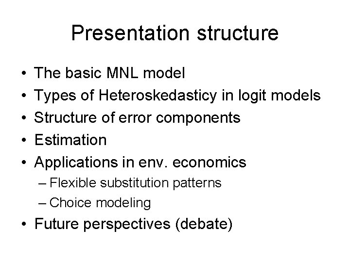
Presentation structure • • • The basic MNL model Types of Heteroskedasticy in logit models Structure of error components Estimation Applications in env. economics – Flexible substitution patterns – Choice modeling • Future perspectives (debate)

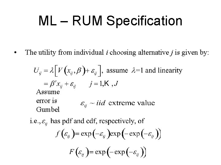
ML – RUM Specification • The utility from individual i choosing alternative j is given by: Assume error is Gumbel i. e. ,

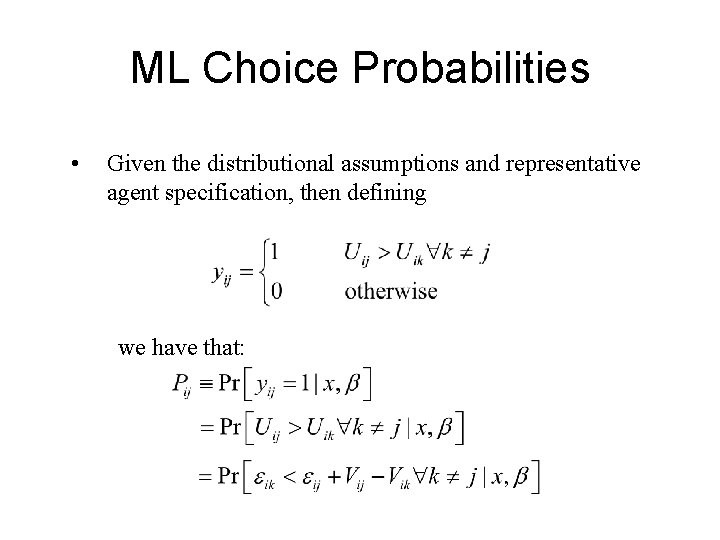
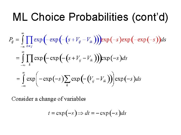
ML Choice Probabilities • Given the distributional assumptions and representative agent specification, then defining we have that:

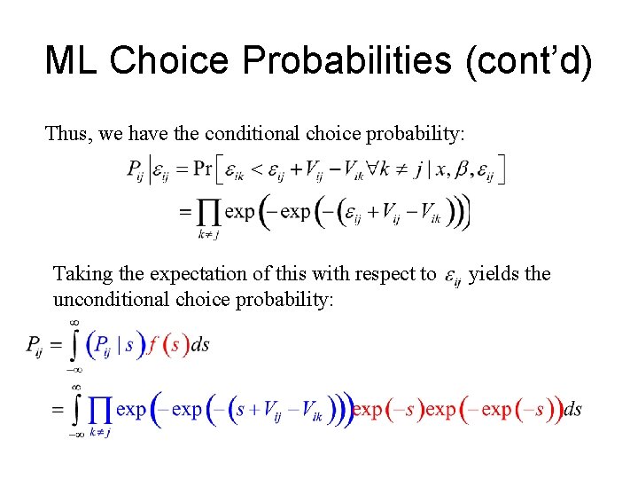
ML Choice Probabilities (cont’d) Thus, we have the conditional choice probability: Taking the expectation of this with respect to unconditional choice probability: yields the

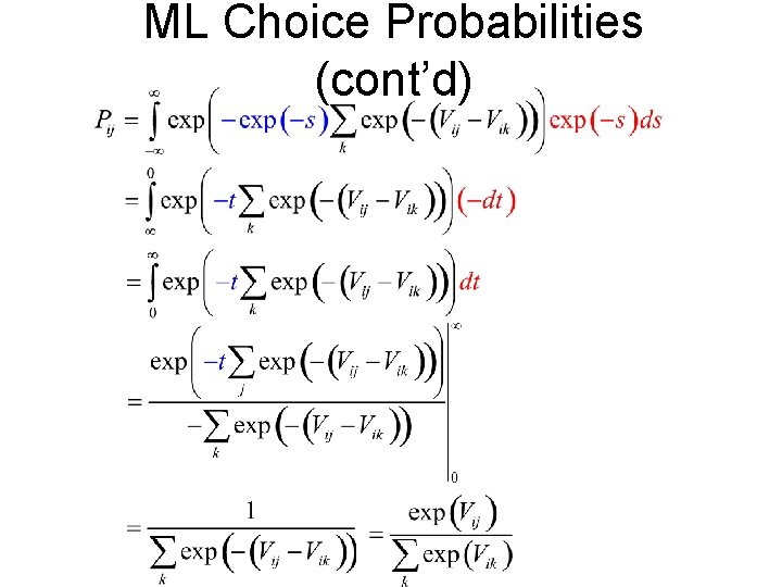
ML Choice Probabilities (cont’d) Consider a change of variables

ML Choice Probabilities (cont’d)

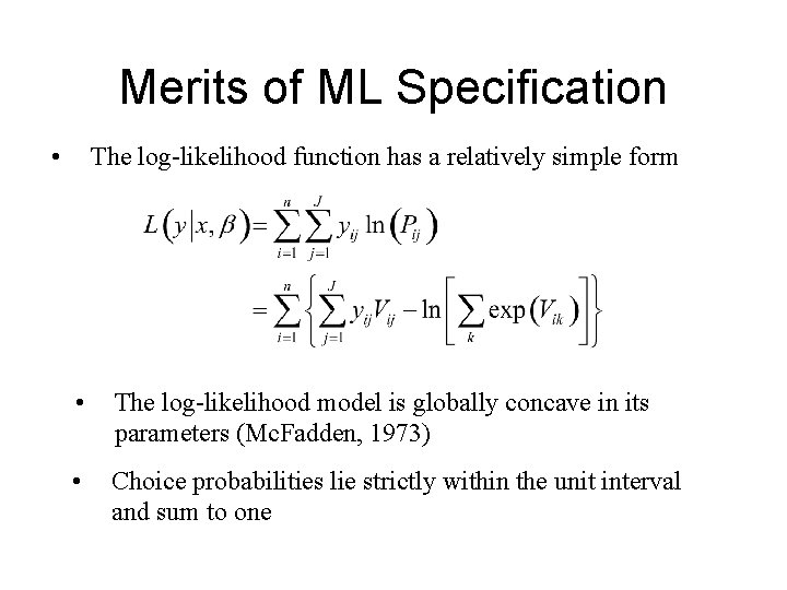
Merits of ML Specification • The log-likelihood function has a relatively simple form • The log-likelihood model is globally concave in its parameters (Mc. Fadden, 1973) • Choice probabilities lie strictly within the unit interval and sum to one

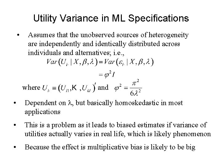
Utility Variance in ML Specifications • Assumes that the unobserved sources of heterogeneity are independently and identically distributed across individuals and alternatives; i. e. , where and • Dependent on , but basically homoskedastic in most applications • This is a problem as it leads to biased estimates if variance of utilities actually varies in real life, which is likely phenomenon • Because the effect is multiplicative bias is likely to be big

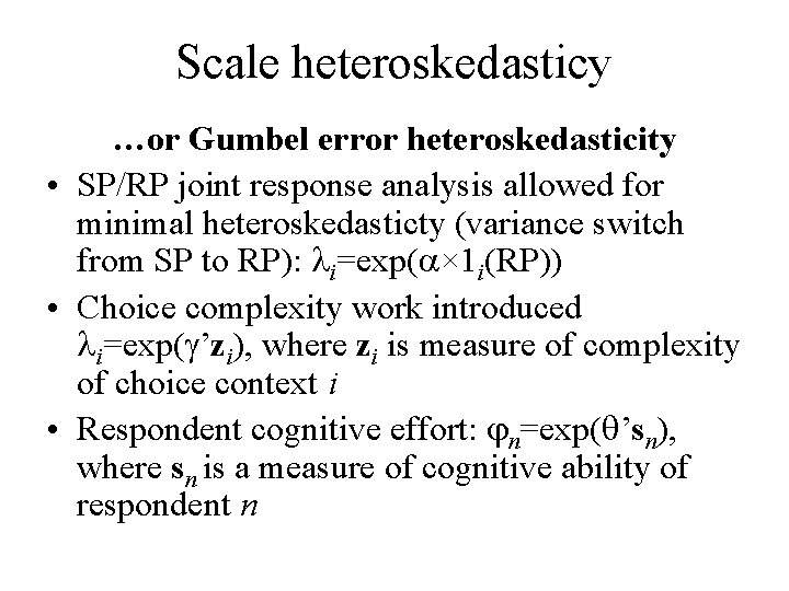
Scale heteroskedasticy …or Gumbel error heteroskedasticity • SP/RP joint response analysis allowed for minimal heteroskedasticty (variance switch from SP to RP): i=exp( × 1 i(RP)) • Choice complexity work introduced i=exp( ’zi), where zi is measure of complexity of choice context i • Respondent cognitive effort: n=exp( ’sn), where sn is a measure of cognitive ability of respondent n

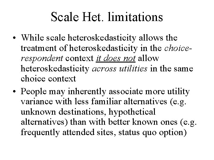
Scale Het. limitations • While scale heteroskedasticity allows the treatment of heteroskedasticity in the choicerespondent context it does not allow heteroskedasticity across utilities in the same choice context • People may inherently associate more utility variance with less familiar alternatives (e. g. unknown destinations, hypothetical alternatives) than with better known ones (e. g. frequently attended sites, status quo option)

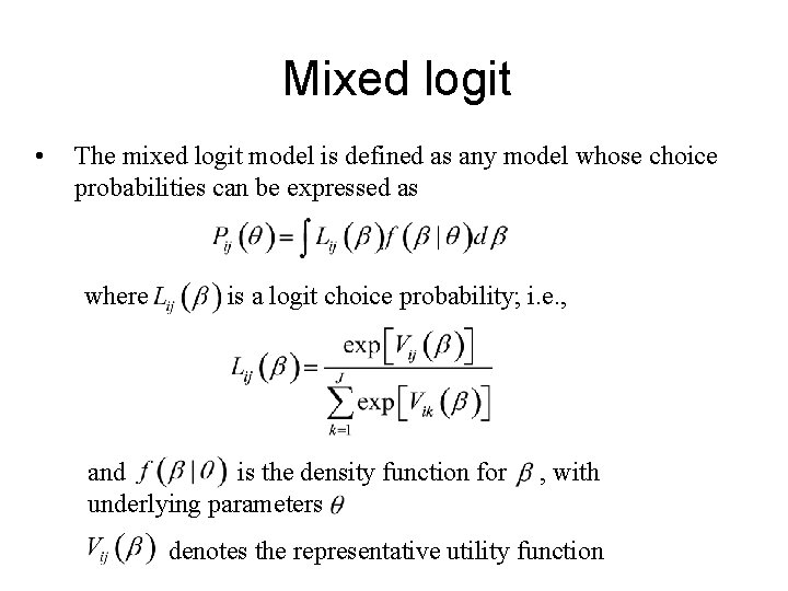
Mixed logit • The mixed logit model is defined as any model whose choice probabilities can be expressed as where is a logit choice probability; i. e. , and is the density function for underlying parameters , with denotes the representative utility function

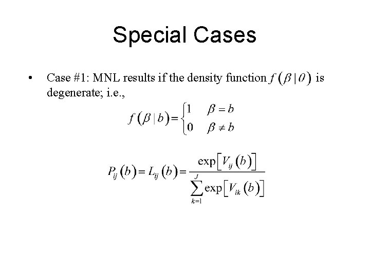
Special Cases • Case #1: MNL results if the density function degenerate; i. e. , is

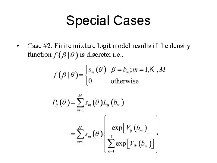
Special Cases • Case #2: Finite mixture logit model results if the density function is discrete; i. e. ,

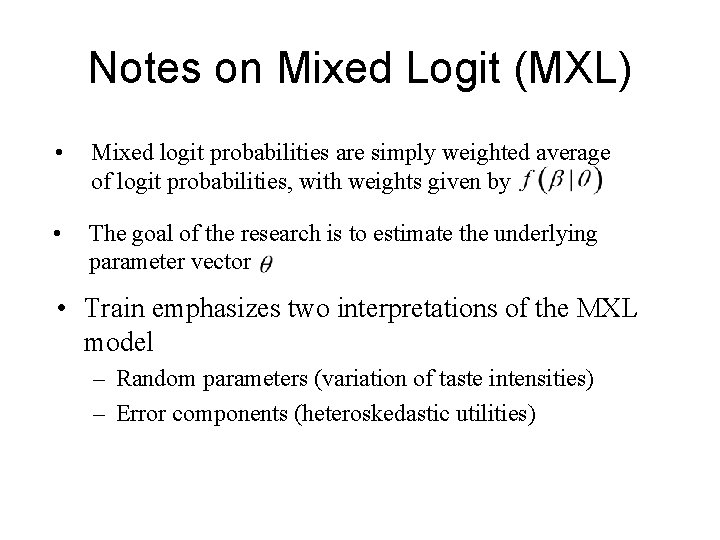
Notes on Mixed Logit (MXL) • Mixed logit probabilities are simply weighted average of logit probabilities, with weights given by • The goal of the research is to estimate the underlying parameter vector • Train emphasizes two interpretations of the MXL model – Random parameters (variation of taste intensities) – Error components (heteroskedastic utilities)

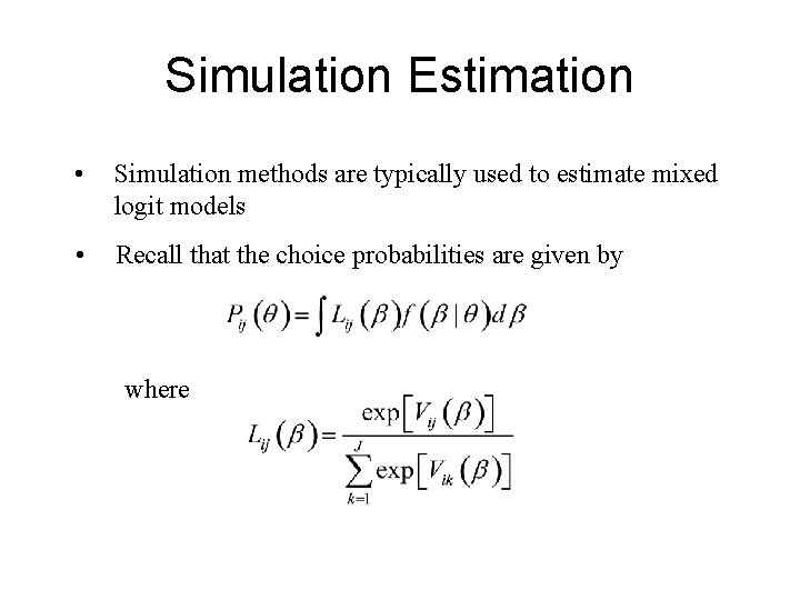
Simulation Estimation • Simulation methods are typically used to estimate mixed logit models • Recall that the choice probabilities are given by where

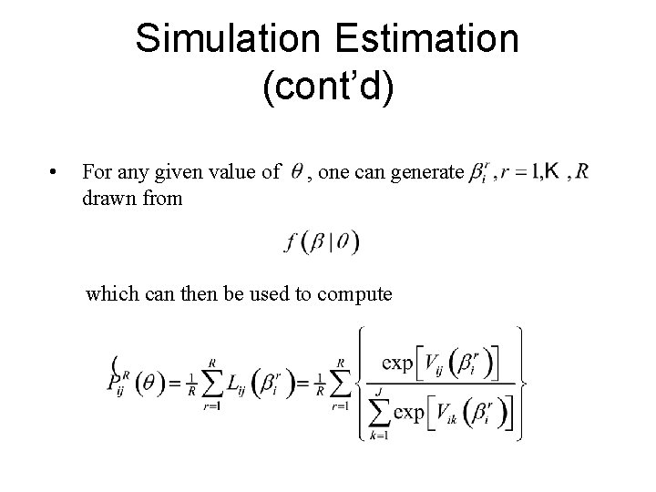
Simulation Estimation (cont’d) • For any given value of drawn from , one can generate which can then be used to compute

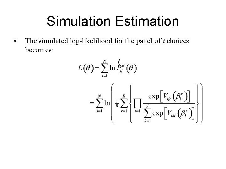
Simulation Estimation • The simulated log-likelihood for the panel of t choices becomes:

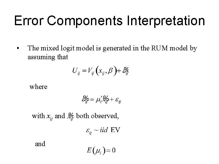
Error Components Interpretation • The mixed logit model is generated in the RUM model by assuming that where with xij and both observed,

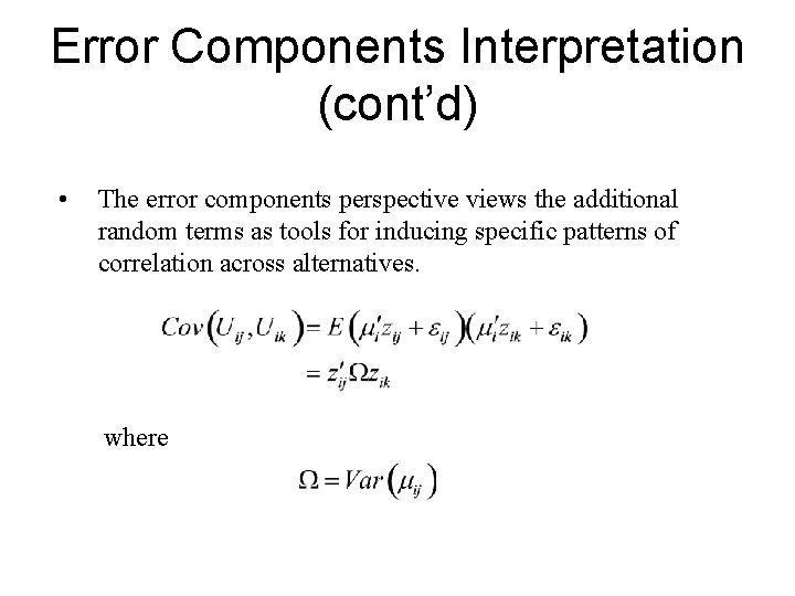
Error Components Interpretation (cont’d) • The error components perspective views the additional random terms as tools for inducing specific patterns of correlation across alternatives. where

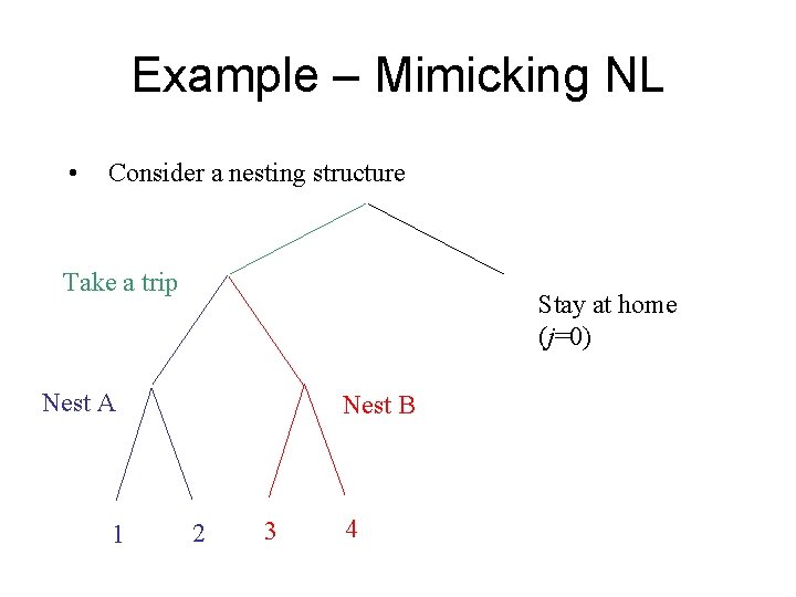
Example – Mimicking NL • Consider a nesting structure Take a trip Stay at home (j=0) Nest A 1 Nest B 2 3 4

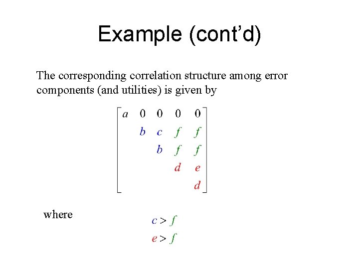
Example (cont’d) The corresponding correlation structure among error components (and utilities) is given by where

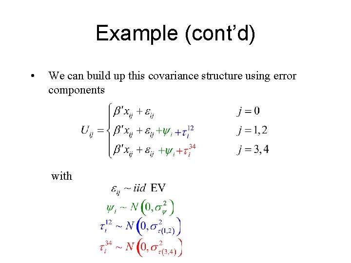
Example (cont’d) • We can build up this covariance structure using error components with

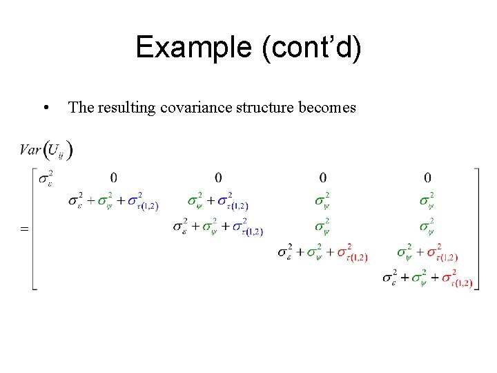
Example (cont’d) • The resulting covariance structure becomes

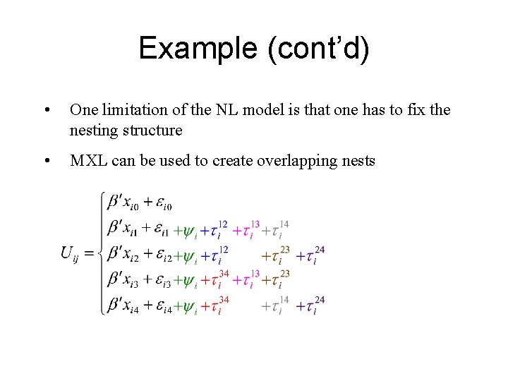
Example (cont’d) • One limitation of the NL model is that one has to fix the nesting structure • MXL can be used to create overlapping nests

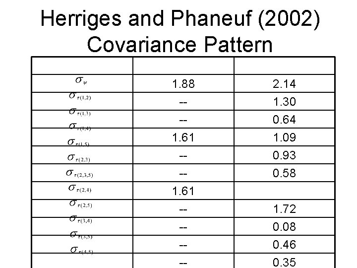
Herriges and Phaneuf (2002) Covariance Pattern 1. 88 --- 2. 14 1. 30 0. 64 1. 61 ----- 1. 09 0. 93 0. 58 1. 72 0. 08 0. 46 0. 35

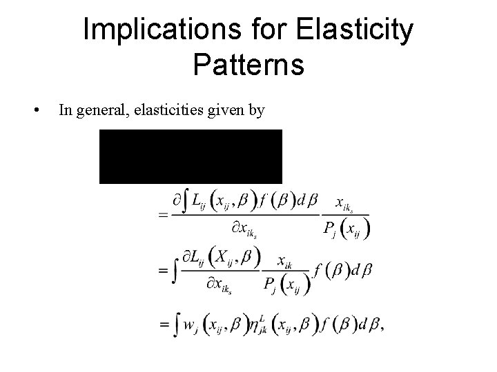
Implications for Elasticity Patterns • In general, elasticities given by

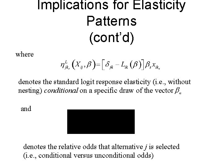
Implications for Elasticity Patterns (cont’d) where denotes the standard logit response elasticity (i. e. , without nesting) conditional on a specific draw of the vector and denotes the relative odds that alternative j is selected (i. e. , conditional versus unconditional odds)

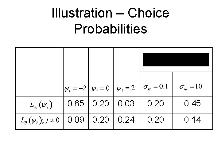
Illustration – Choice Probabilities 0. 65 0. 20 0. 03 0. 20 0. 45 0. 09 0. 20 0. 24 0. 20 0. 14

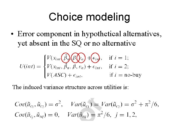
Choice modeling • Error component in hypothetical alternatives, yet absent in the SQ or no alternative The induced variance structure across utilities is:

Effect • Fairly general result that it improves fit while requiring few additional parameters (only st. dev. of err. comp. ) • It can be decomposed by socio-economics covariates (e. g. spread of error varies across segments of respondents)

Adoption and state of practice • Error component estimators have now been incorporated in commercial software (e. g. Nlogit 4) • Given their properties and the flexibility they afford they are likely to be increasingly used in practice