ERICSSON MEETS SMID ANALYSE April 2011 Agenda 4

ERICSSON MEETS SMID ANALYSE April, 2011

Agenda › 4 th April – Ericsson presentation – Statistical tools in manufacturing – DMAIC/IDDOV › 7 th April – Define – Measure › 11 th April – Analyze › 14 th April – Implement – Control 04. Analyze | Ericsson Confidential | 2011 -04 -04 | Page 2 (49)

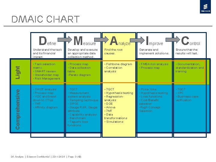
DMAIC Chart Comprehensive Light D efine M easure A nalyze I mprove C ontrol Understand the task and its financial impact. Develop and execute an appropriate data collection method. Find the root causes. Generate and implement solutions. Ensure that the results will last. • Task selection matrix • SMART review • Stakeholder map • Risk Management • Process map • Data collection table • Pareto diagram • Fishbone diagram • Correlation analysis • FMEA risk analysis • Process map • Documentation, standardization and training • SWOT analysis • Process map • VOC and break down to CTQs • 7 MT • Affinity diagram • 7 QCT • Measurement system analysis • Sampling technique • SIPOC • Gauge R&R, Gauge attribute • Capability analysis • Benchmark • Tagushi loss functions • 7 QCT • Hypothesis testing • Regressionanalysis • DOE • Anova • 7 MT • Data transformations • Simulations • Poka-Yoke • Hypothesis testing • Loss functions • Cost/Benefit selection • Pugh Concept Selection • 7 QCT • SPC • Business case verification 04. Analyze | Ericsson Confidential | 2011 -04 -04 | Page 3 (49)

CAPABILITY

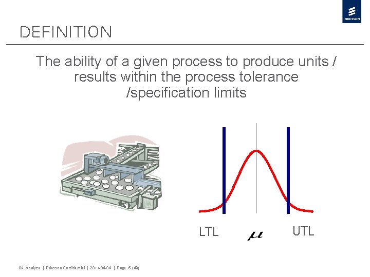
Definition The ability of a given process to produce units / results within the process tolerance /specification limits LTL 04. Analyze | Ericsson Confidential | 2011 -04 -04 | Page 5 (49) UTL

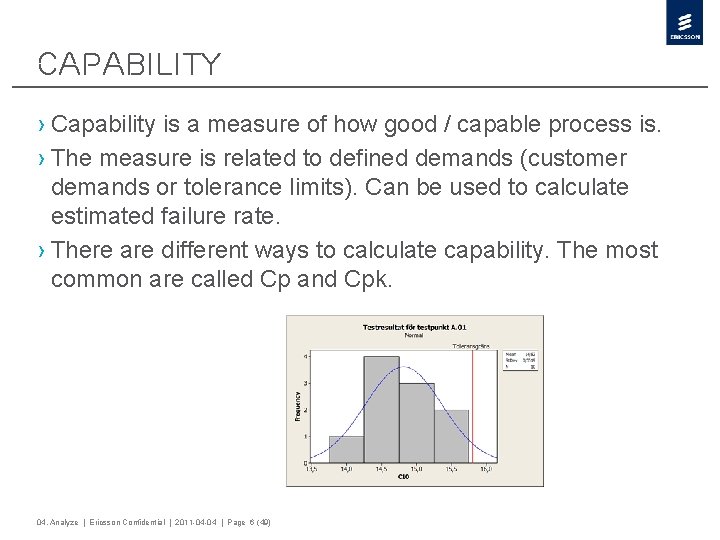
Capability › Capability is a measure of how good / capable process is. › The measure is related to defined demands (customer demands or tolerance limits). Can be used to calculate estimated failure rate. › There are different ways to calculate capability. The most common are called Cp and Cpk. 04. Analyze | Ericsson Confidential | 2011 -04 -04 | Page 6 (49)

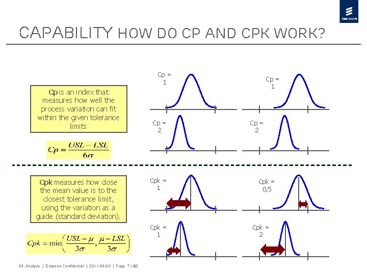
CAPABILITY how do Cp and Cpk work? Cp = 1 Cp is an index that measures how well the process variation can fit within the given tolerance limits Cpk measures how close the mean value is to the closest tolerance limit, using the variation as a guide (standard deviation). Cp = 2 Cpk = 1 04. Analyze | Ericsson Confidential | 2011 -04 -04 | Page 7 (49) Cp = 1 Cp = 2 Cpk = 0, 5 Cpk = 2

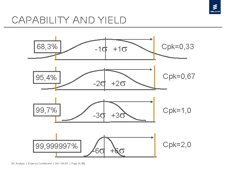
Capability and Yield 68, 3% 95, 4% 99, 7% 99, 999997% 04. Analyze | Ericsson Confidential | 2011 -04 -04 | Page 8 (49) -1 +1 -2 +2 Cpk=0, 33 Cpk=0, 67 -3 +3 Cpk=1, 0 -6 +6 Cpk=2, 0

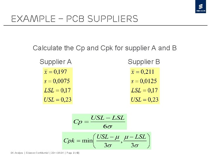
Example – PCB suppliers Calculate the Cp and Cpk for supplier A and B Supplier A 04. Analyze | Ericsson Confidential | 2011 -04 -04 | Page 9 (49) Supplier B

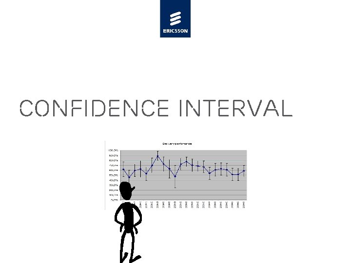
CONFIDENCE INTERVAL

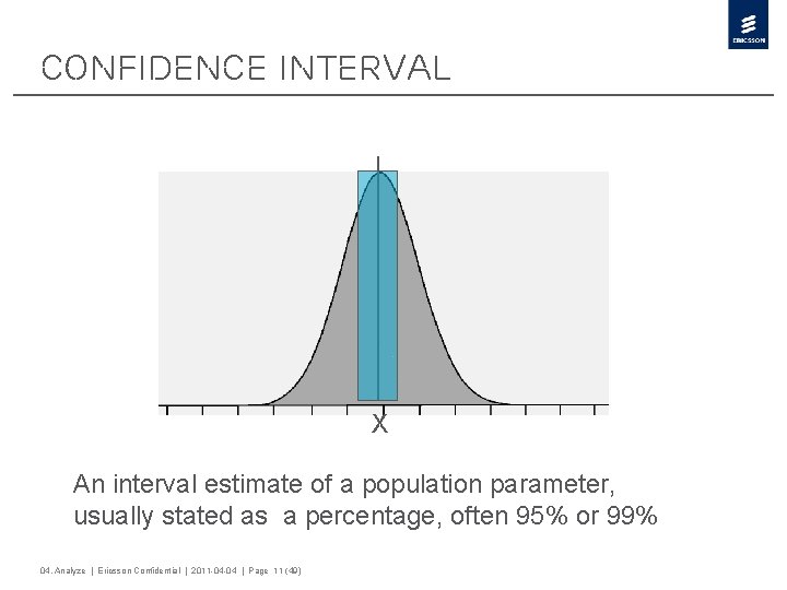
Confidence Interval X An interval estimate of a population parameter, usually stated as a percentage, often 95% or 99% 04. Analyze | Ericsson Confidential | 2011 -04 -04 | Page 11 (49)

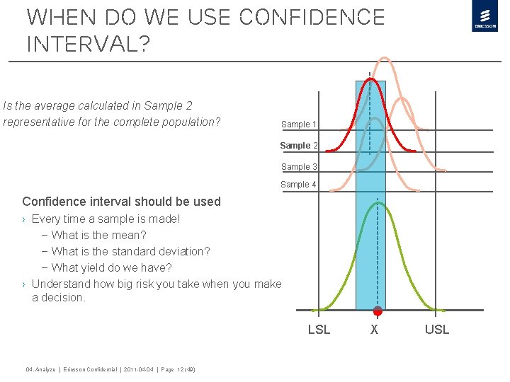
When do we use Confidence Interval? Is the average calculated in Sample 2 representative for the complete population? Sample 1 Sample 2 Sample 3 Sample 4 Confidence interval should be used › Every time a sample is made! – What is the mean? – What is the standard deviation? – What yield do we have? › Understand how big risk you take when you make a decision. LSL 04. Analyze | Ericsson Confidential | 2011 -04 -04 | Page 12 (49) X USL

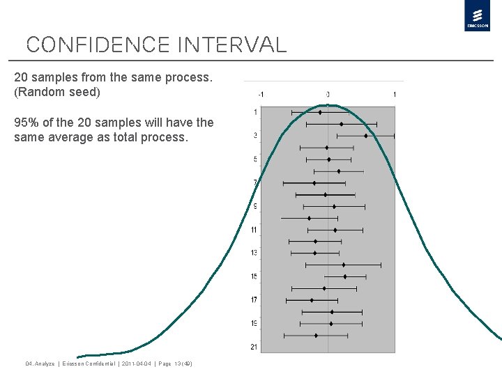
Confidence interval 20 samples from the same process. (Random seed) 95% of the 20 samples will have the same average as total process. 04. Analyze | Ericsson Confidential | 2011 -04 -04 | Page 13 (49)

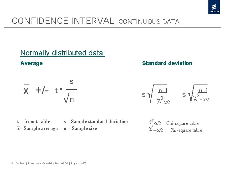
Confidence interval, continuous data Normally distributed data: Average x +/- Standard deviation s t* t = from t-table x= Sample average n s = Sample standard deviation n = Sample size 04. Analyze | Ericsson Confidential | 2011 -04 -04 | Page 14 (49) S* n-1 Chi-square table

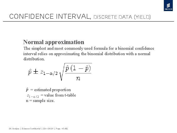
Confidence interval, discrete data (Yield) Normal approximation The simplest and most commonly used formula for a binomial confidence interval relies on approximating the binomial distribution with a normal distribution. = estimated proportion z 1 − α / 2 = value from t-table n = sample size. 04. Analyze | Ericsson Confidential | 2011 -04 -04 | Page 15 (49)

Compare performance? 04. Analyze | Ericsson Confidential | 2011 -04 -04 | Page 16 (49)

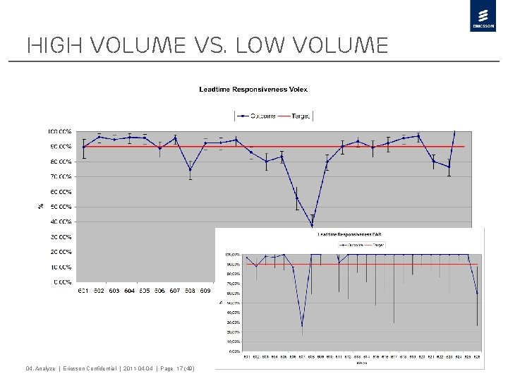
High volume vs. low volume 04. Analyze | Ericsson Confidential | 2011 -04 -04 | Page 17 (49)

CORRELATION REGRESSION

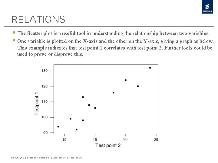
Relations § The Scatter plot is a useful tool in understanding the relationship between two variables. § One variable is plotted on the X-axis and the other on the Y-axis, giving a graph as below. This example indicates that test point 1 correlates with test point 2. Further tools could be used to prove or disprove this. 04. Analyze | Ericsson Confidential | 2011 -04 -04 | Page 19 (49)

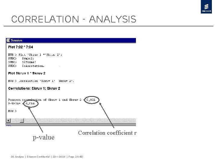
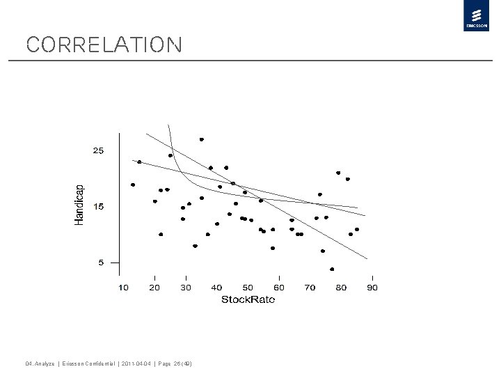
Correlation › Correlation is a technique for investigating the relationship between two quantitative, continuous variables. › Correlation is the degree or extent of the relationship between two variables. – If the value of one variable increases when the value of the other increases, they are said to be positively correlated. – If the value of one variable decreases when the value other variable is increasing it is said to be negatively correlated. – If one variable does not affect the other they are considered to not be correlated. › The correlation coefficient quantifies the degree of linear association between two variables. It is typically denoted by r and will have a value ranging between -1 and positive 1. 04. Analyze | Ericsson Confidential | 2011 -04 -04 | Page 20 (49)

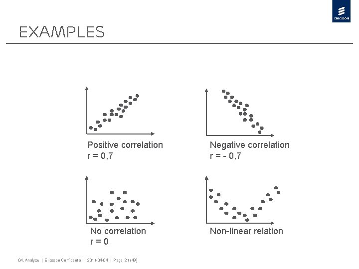
Examples Positive correlation r = 0, 7 No correlation r=0 04. Analyze | Ericsson Confidential | 2011 -04 -04 | Page 21 (49) Negative correlation r = - 0, 7 Non-linear relation

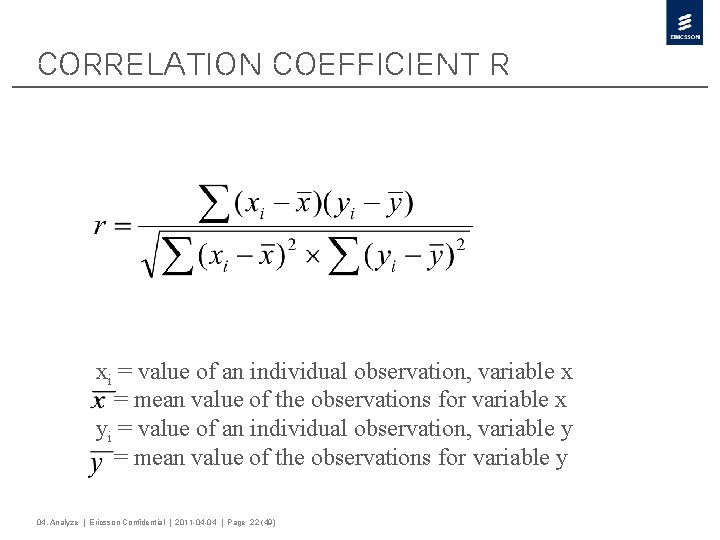
Correlation coefficient r xi = value of an individual observation, variable x = mean value of the observations for variable x yi = value of an individual observation, variable y = mean value of the observations for variable y 04. Analyze | Ericsson Confidential | 2011 -04 -04 | Page 22 (49)

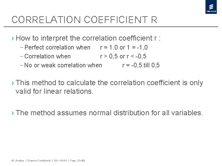
Correlation coefficient r › How to interpret the correlation coefficient r : – Perfect correlation when r = 1. 0 or 1 = -1, 0 – Correlation when r > 0, 5 or r < -0, 5 – No or weak correlation when r = -0, 5 till 0, 5 › This method to calculate the correlation coefficient is only valid for linear relations. › The method assumes normal distribution for all variables. 04. Analyze | Ericsson Confidential | 2011 -04 -04 | Page 23 (49)

Correlation - analysis p-value Correlation coefficient r 04. Analyze | Ericsson Confidential | 2011 -04 -04 | Page 24 (49)

REGRESSION

Correlation 04. Analyze | Ericsson Confidential | 2011 -04 -04 | Page 26 (49)

Definition The data should empirically quantify, through a mathematical model, the relationship that exists between the response variable and influencing factors 04. Analyze | Ericsson Confidential | 2011 -04 -04 | Page 27 (49)

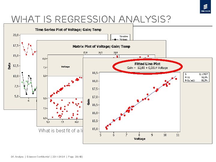
What is regression analysis? › Is there a relation between › Gain, Temperature and › Voltage? › If it is, can it be describe in a › formula? Y=f(x) What is best fit of a line between Gain and Voltage? 04. Analyze | Ericsson Confidential | 2011 -04 -04 | Page 28 (49)

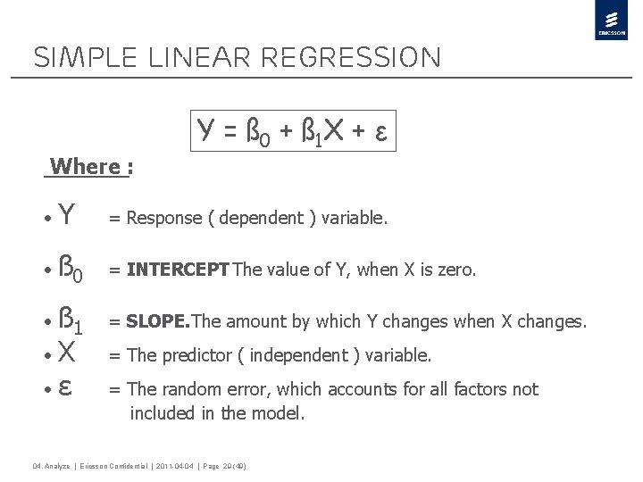
Simple Linear Regression Y = ß 0 + ß 1 X + ε Where : • Y = Response ( dependent ) variable. • ß 0 = INTERCEPT. The value of Y, when X is zero. ß 1 • X • ε • = SLOPE. The amount by which Y changes when X changes. = The predictor ( independent ) variable. = The random error, which accounts for all factors not included in the model. 04. Analyze | Ericsson Confidential | 2011 -04 -04 | Page 29 (49)

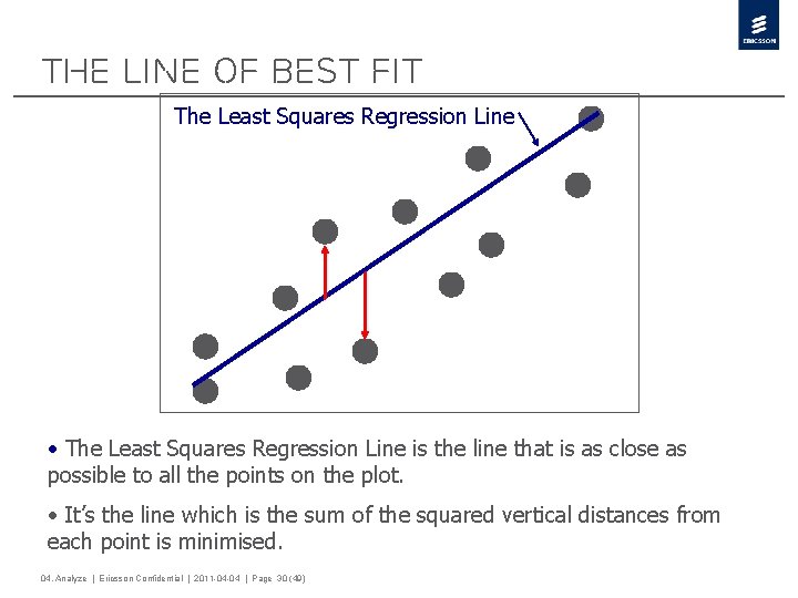
The Line of Best Fit The Least Squares Regression Line • The Least Squares Regression Line is the line that is as close as possible to all the points on the plot. • It’s the line which is the sum of the squared vertical distances from each point is minimised. 04. Analyze | Ericsson Confidential | 2011 -04 -04 | Page 30 (49)

Collecting data › Measurement of X is assumed to be precise. › In regression it is assumed that the random variation occurs in Y as X is changed. › The regression model will only be a predictor of behaviour within the data range, I. e. extrapolation is usually not allowed › As a rule of thumb- should have at least 30 data points to perform a regression analysis 04. Analyze | Ericsson Confidential | 2011 -04 -04 | Page 32 (49)

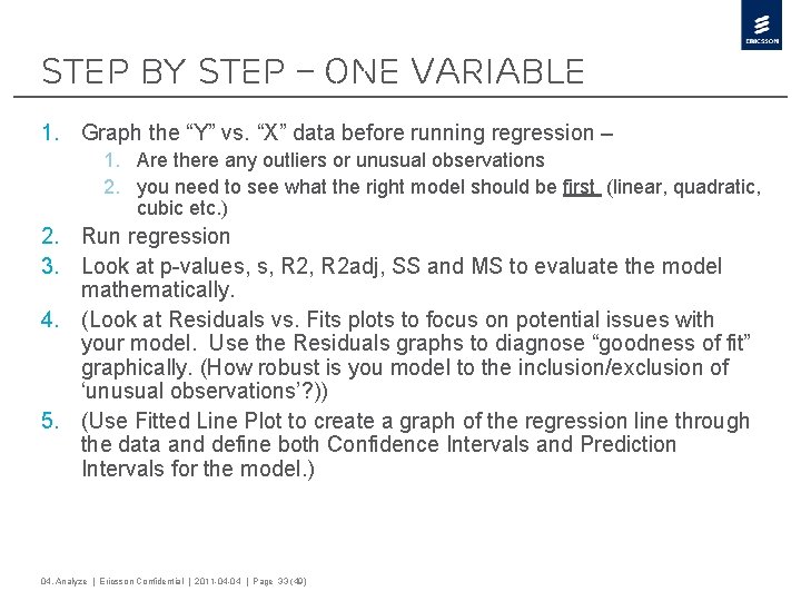
Step by step – One Variable 1. Graph the “Y” vs. “X” data before running regression – 1. Are there any outliers or unusual observations 2. you need to see what the right model should be first (linear, quadratic, cubic etc. ) 2. Run regression 3. Look at p-values, s, R 2 adj, SS and MS to evaluate the model mathematically. 4. (Look at Residuals vs. Fits plots to focus on potential issues with your model. Use the Residuals graphs to diagnose “goodness of fit” graphically. (How robust is you model to the inclusion/exclusion of ‘unusual observations’? )) 5. (Use Fitted Line Plot to create a graph of the regression line through the data and define both Confidence Intervals and Prediction Intervals for the model. ) 04. Analyze | Ericsson Confidential | 2011 -04 -04 | Page 33 (49)

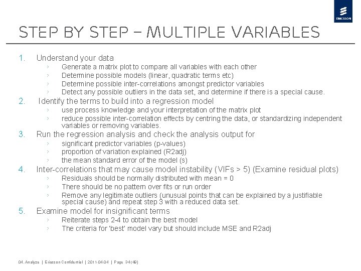
Step by step – MULTIPLE Variables 1. Understand your data › › 2. Identify the terms to build into a regression model › › 3. significant predictor variables (p-values) proportion of variation explained (R 2 adj) the mean standard error of the model (s) Inter-correlations that may cause model instability (VIFs > 5) (Examine residual plots) › › › 5. use process knowledge and your interpretation of the matrix plot reduce possible inter-correlation effects by centring the data, or standardizing independent variables or removing variables. Run the regression analysis and check the analysis output for › › › 4. Generate a matrix plot to compare all variables with each other Determine possible models (linear, quadratic terms etc) Determine possible inter-correlations amongst predictor variables Detect any possible outliers in the data set, and determine if there is a special cause. Residuals should be normally distributed with mean = 0 There should be no pattern over fits or run order Remove any legitimate outliers (unusual points that can be explained by a justifiable special cause) and repeat step 3 with a reduced data set. Examine model for insignificant terms › › Reiterate steps 2 -4 to obtain the best model The criteria for ‘best’ model vary but should include MSE and R 2 adj 04. Analyze | Ericsson Confidential | 2011 -04 -04 | Page 34 (49)

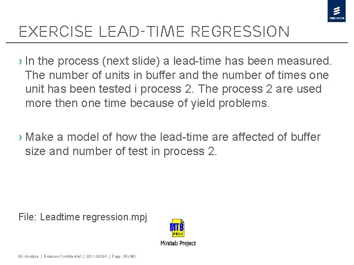
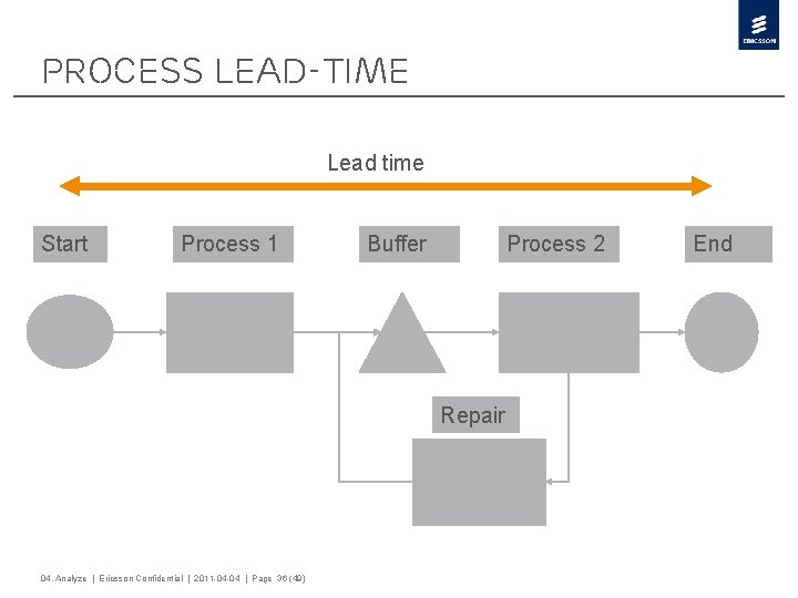
Exercise Lead-time regression › In the process (next slide) a lead-time has been measured. The number of units in buffer and the number of times one unit has been tested i process 2. The process 2 are used more then one time because of yield problems. › Make a model of how the lead-time are affected of buffer size and number of test in process 2. File: Leadtime regression. mpj 04. Analyze | Ericsson Confidential | 2011 -04 -04 | Page 35 (49)

Process Lead-time Lead time Start Process 1 Buffer Process 2 Repair 04. Analyze | Ericsson Confidential | 2011 -04 -04 | Page 36 (49) End

MEASUREMENT SYSTEM ANALYSIS GAGE R&R

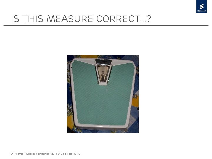
Is this measure correct…? 04. Analyze | Ericsson Confidential | 2011 -04 -04 | Page 38 (49)

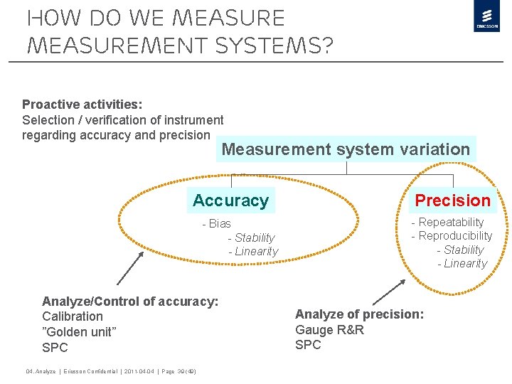
How do we measurement systems? Proactive activities: Selection / verification of instrument regarding accuracy and precision Measurement system variation Accuracy - Bias - Stability - Linearity Analyze/Control of accuracy: Calibration ”Golden unit” SPC 04. Analyze | Ericsson Confidential | 2011 -04 -04 | Page 39 (49) Precision - Repeatability - Reproducibility - Stability - Linearity Analyze of precision: Gauge R&R SPC

Measurement uncertainty › Gauge R&R (Repeatability & Reproducibility) study › A selection of at least 5 production parts measured at least 2 times by at least 2 different appraisers (operators, test stations etc) › R&R is calculated and compared to the total variation (including part to part variation) and total tolerance (specification limits) to assess if the measurement system is acceptable 04. Analyze | Ericsson Confidential | 2011 -04 -04 | Page 40 (49)

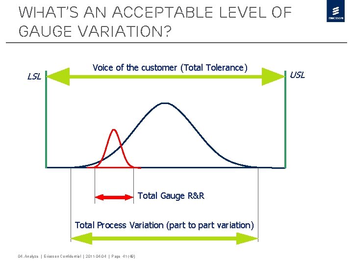
What’s an acceptable level of Gauge Variation? LSL Voice of the customer (Total Tolerance) Total Gauge R&R Total Process Variation (part to part variation) 04. Analyze | Ericsson Confidential | 2011 -04 -04 | Page 41 (49) USL

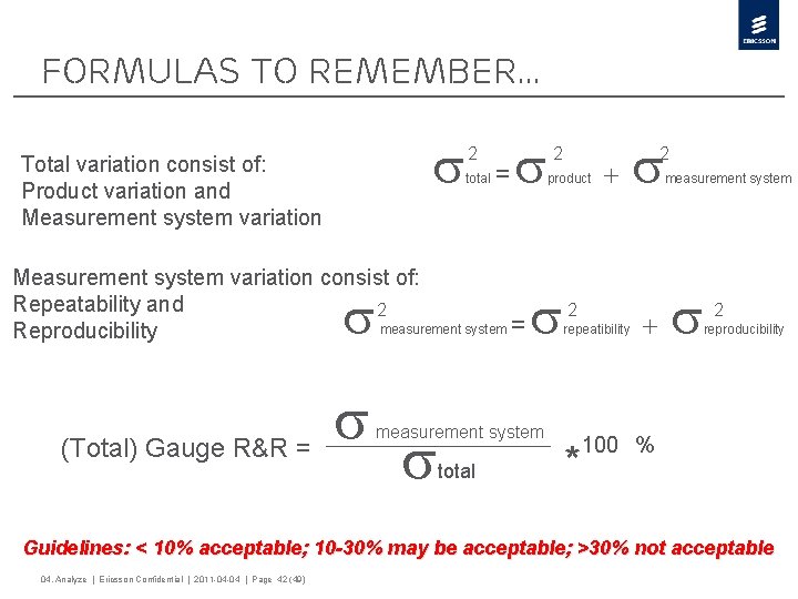
formulas to remember… = + 2 Total variation consist of: Product variation and Measurement system variation total Measurement system variation consist of: Repeatability and 2 measurement system = Reproducibility (Total) Gauge R&R = 2 product measurement system total 2 2 + repeatibility * measurement system 2 reproducibility 100 % Guidelines: < 10% acceptable; 10 -30% may be acceptable; >30% not acceptable 04. Analyze | Ericsson Confidential | 2011 -04 -04 | Page 42 (49)

Gage R&R Analyze - Minitab › Example › One Yellow Belt in CDU production wants to check for variation in the test stations. › The production line has 3 test stations and he wants to do an Gage R&R analyze. › 3 approved CDU are tested 3 times in all 3 test stations. › The test program consists of 2 test points 04. Analyze | Ericsson Confidential | 2011 -04 -04 | Page 43 (49)

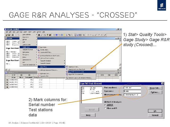
Gage R&R Analyses - “Crossed” 1) Stat> Quality Tools> Gage Study> Gage R&R study (Crossed). . . 2) Mark columns for: Serial number Test stations data 04. Analyze | Ericsson Confidential | 2011 -04 -04 | Page 44 (49)

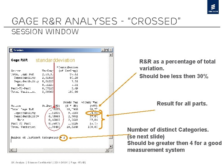
Gage R&R Analyses - “Crossed” Session Window standarddeviation R&R as a percentage of total variation. Should bee less then 30% Result for all parts. Number of distinct Categories. (se next slide) Should be greater then 4 for a good measurement system 04. Analyze | Ericsson Confidential | 2011 -04 -04 | Page 45 (49)

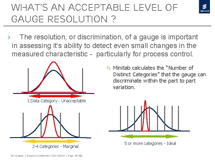
What’s an acceptable level of Gauge resolution ? › The resolution, or discrimination, of a gauge is important in assessing it’s ability to detect even small changes in the measured characteristic - particularly for process control. n Minitab calculates the “Number of Distinct Categories” that the gauge can discriminate within the part to part variation. 1 Data Category - Unacceptable 2 -4 Categories - Marginal 04. Analyze | Ericsson Confidential | 2011 -04 -04 | Page 46 (49) 5 or more categories - Ideal

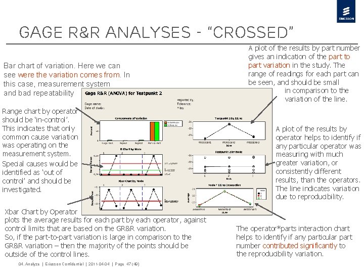
Gage R&R Analyses - “Crossed” Bar chart of variation. Here we can see were the variation comes from. In this case, measurement system and bad repeatability Range chart by operator should be ‘in-control’. This indicates that only common cause variation was operating on the measurement system. Special causes would be identified as ‘out of control’ and should be investigated. Xbar Chart by Operator plots the average results for each part by each operator, against control limits that are based on the GR&R variation. So, if the part-to-part variation is large in comparison to the GR&R variation – then the majority of the points should be outside of the control lines. 04. Analyze | Ericsson Confidential | 2011 -04 -04 | Page 47 (49) A plot of the results by part number gives an indication of the part to part variation in the study. The range of readings for each part can be seen, and should be small in comparison to the variation of the line. A plot of the results by operator helps to identify if any particular operator was measuring with much greater variation, or consistently different results, than the operators. The line indicates variation due to reproducibility. The operator*parts interaction chart helps to identify if any particular part number contributed significantly to the reproducibility variation.

Rules to remember › Always randomise the runs › Use the actual gauge, appraisers and production parts. › Ensure the parts represent the full range of output. › Complete the study in the production environment. › Label the parts discreetly & avoid the appraiser seeing the part labels › Have a facilitator who records the results › Check for out of control records on a range chart. › Be aware of within part variation 04. Analyze | Ericsson Confidential | 2011 -04 -04 | Page 48 (49)

04. Analyze | Ericsson Confidential | 2011 -04 -04 | Page 49 (49)