Equity Risk Credit Risk Default Correlation and Corporate

Equity Risk, Credit Risk, Default Correlation, and Corporate Sustainability Dan di. Bartolomeo Northfield Information Services February 2011

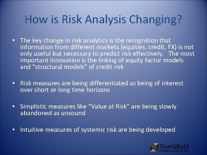
How is Risk Analysis Changing? • The key change in risk analytics is the recognition that information from different markets (equities, credit, FX) is not only useful but necessary to predict risk effectively. The most important innovation is the linking of equity factor models and “structural models” of credit risk • Risk measures are being differentiated as being of interest over short or long time horizons • Simplistic measures like “Value at Risk” are being slowly abandoned as unsound • Intuitive measures of systemic risk are being developed

Goals for this Presentation Illustrate how equity factor risk models and structural models of credit risk can be linked to provide consistent measures of equity risk, default risk and default correlation Introduce a quantitative measure of the “sustainability” of firms Describe results in an empirical analysis of all US listed equities from 1992 to present Show that common conception of “sustainable” investing is confirmed in these results Illustrate an alternative use of this method as a way to define the level of systemic risk to developed economies

Basic Contingent Claims Literature Merton (1974) poses the equity of a firm as a European call option on the firm’s assets, with a strike price equal to the face value of the firm’s debt Alternatively, lenders are short a put on the firm assets Default can occur only at debt maturity Black and Cox (1976) provide a “first passage” model Default can occur before debt maturity Firm extinction is assumed if asset values hit a boundary value (i. e. specified by bond covenants) Leland (1994) and Leland Toft (1996) Account for the tax deductibility of interest payments and costs of bankruptcy Estimate boundary value as where equity value is maximized subject to bankruptcy

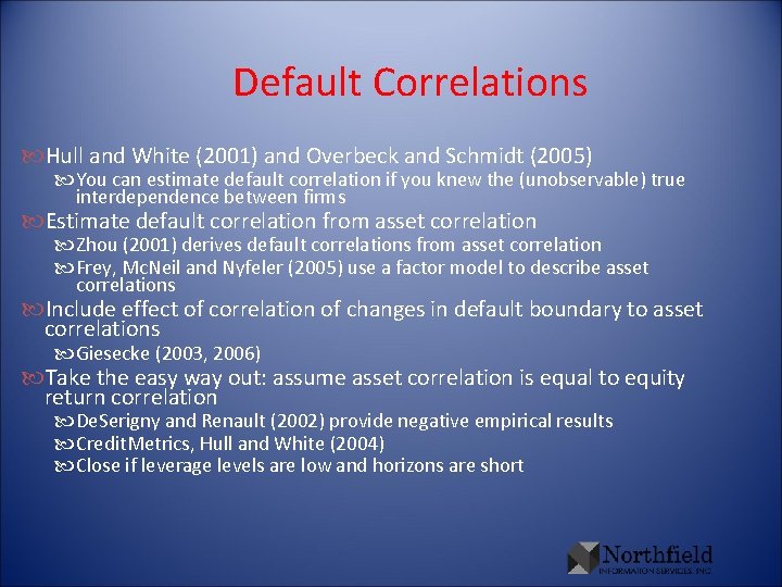
Default Correlations Hull and White (2001) and Overbeck and Schmidt (2005) You can estimate default correlation if you knew the (unobservable) true interdependence between firms Estimate default correlation from asset correlation Zhou (2001) derives default correlations from asset correlation Frey, Mc. Neil and Nyfeler (2005) use a factor model to describe asset correlations Include effect of correlation of changes in default boundary to asset correlations Giesecke (2003, 2006) Take the easy way out: assume asset correlation is equal to equity return correlation De. Serigny and Renault (2002) provide negative empirical results Credit. Metrics, Hull and White (2004) Close if leverage levels are low and horizons are short

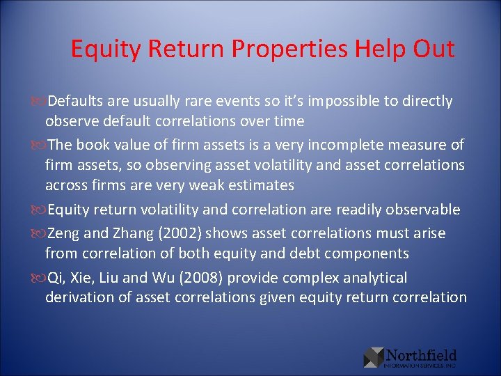
Equity Return Properties Help Out Defaults are usually rare events so it’s impossible to directly observe default correlations over time The book value of firm assets is a very incomplete measure of firm assets, so observing asset volatility and asset correlations across firms are very weak estimates Equity return volatility and correlation are readily observable Zeng and Zhang (2002) shows asset correlations must arise from correlation of both equity and debt components Qi, Xie, Liu and Wu (2008) provide complex analytical derivation of asset correlations given equity return correlation

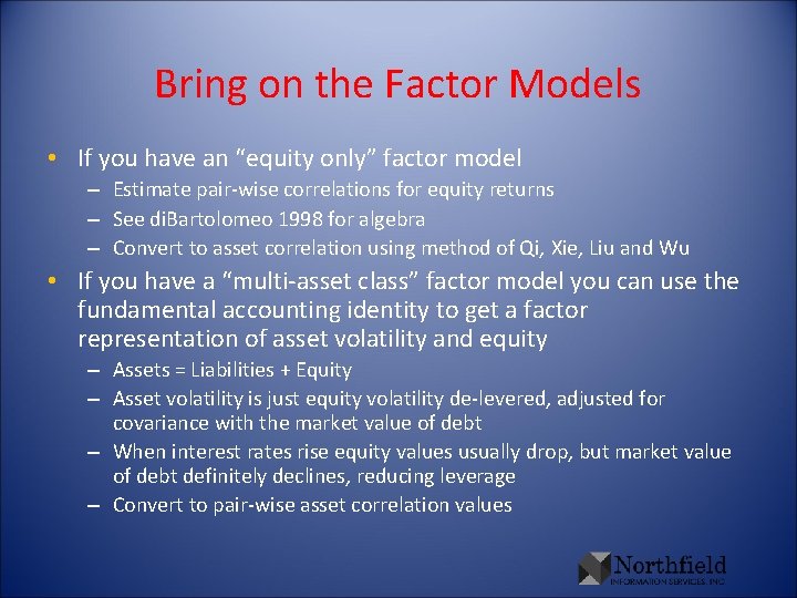
Bring on the Factor Models • If you have an “equity only” factor model – Estimate pair-wise correlations for equity returns – See di. Bartolomeo 1998 for algebra – Convert to asset correlation using method of Qi, Xie, Liu and Wu • If you have a “multi-asset class” factor model you can use the fundamental accounting identity to get a factor representation of asset volatility and equity – Assets = Liabilities + Equity – Asset volatility is just equity volatility de-levered, adjusted for covariance with the market value of debt – When interest rates rise equity values usually drop, but market value of debt definitely declines, reducing leverage – Convert to pair-wise asset correlation values

In Theory, We’re Ready to Go With asset volatility and correlations estimated we can use our preferred structural model to estimate default probability of a firm Use method from Zhou to convert asset correlations to default correlations We can now produce joint default probabilities across firms However there are some pretty restrictive assumptions Firm must have debt today Firm must have positive book value today Balance sheet leverage must stay fixed in the future

Reverse the Concept: Sustainability • Instead of trying to estimate how likely it is that firm goes bankrupt, let’s reverse the logic • We will actually estimate the “market implied expected life” of firms using contingent claims analysis • Firms with no debt can now be included since it is possible that they get some debt in the future and default on that • A quantitative measure of the fundamental and “social” concept of sustainability

Our Basic Option Pricing Exercise Underlying is the firm’s assets with asset volatility determined from the factor model as previously described Solve numerically for the “implied expiration date” of the option that equates the option value to the stock price Market implied expected life of the firm Include a term structure of interest rates so that as the implied expiration date moves around, the interest rate changes appropriately If you choose Black-Scholes as your option model, then you can solve BS for the implied time to expiration using a Taylor series approximation More complex option models allow for stochastic interest rates

Filling in with “Distance to Run” For firm’s with no debt or negative book value, we simply assume that non-survival will be coincident with stock price to zero, since a firm with a positive stock price should be able to sell shares to raise cash to pay debt If you have a stock with 40% a year volatility you need a 2. 5 standard deviation event to get a -100 return Convert to probability under your distributional assumption We convert both measures to the median of the distribution of future survival in years What is the number of years such that the probability of firm survival to this point in time is 50/50 Highly skewed distribution so we upper bound at 300 years Z-score the “median of life” for both measures and map the distance to run Z-scores into the “option method” distribution for firms with no debt

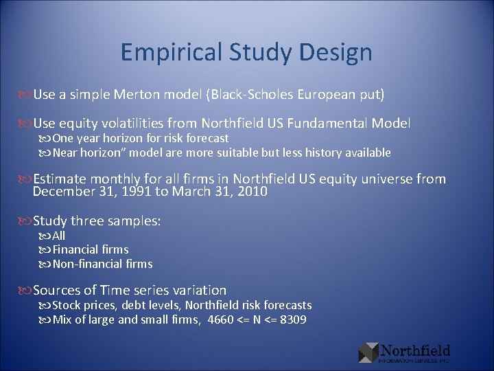
Empirical Study Design Use a simple Merton model (Black-Scholes European put) Use equity volatilities from Northfield US Fundamental Model One year horizon for risk forecast Near horizon” model are more suitable but less history available Estimate monthly for all firms in Northfield US equity universe from December 31, 1991 to March 31, 2010 Study three samples: All Financial firms Non-financial firms Sources of Time series variation Stock prices, debt levels, Northfield risk forecasts Mix of large and small firms, 4660 <= N <= 8309

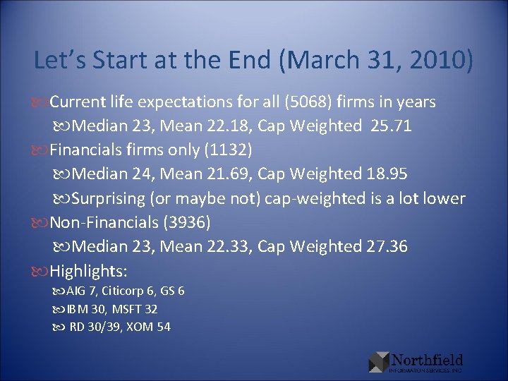
Let’s Start at the End (March 31, 2010) Current life expectations for all (5068) firms in years Median 23, Mean 22. 18, Cap Weighted 25. 71 Financials firms only (1132) Median 24, Mean 21. 69, Cap Weighted 18. 95 Surprising (or maybe not) cap-weighted is a lot lower Non-Financials (3936) Median 23, Mean 22. 33, Cap Weighted 27. 36 Highlights: AIG 7, Citicorp 6, GS 6 IBM 30, MSFT 32 RD 30/39, XOM 54

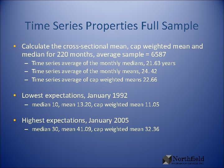
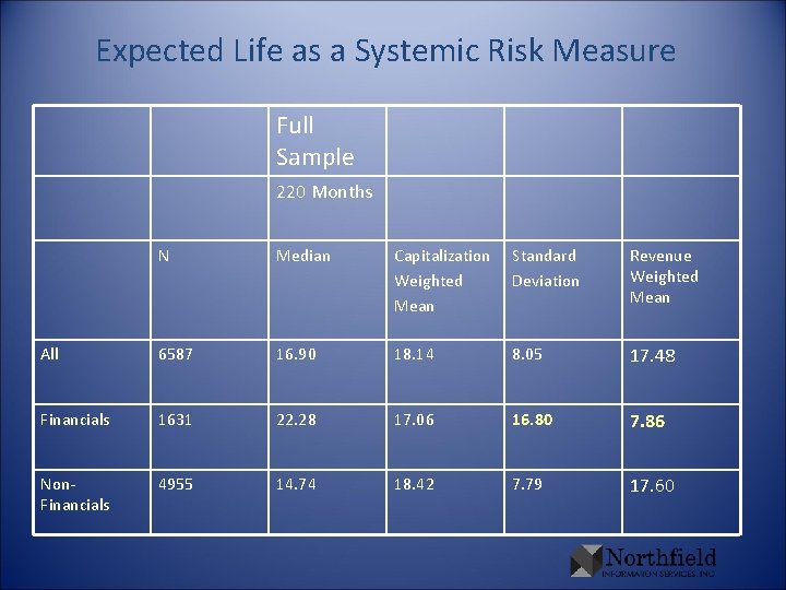
Time Series Properties Full Sample • Calculate the cross-sectional mean, cap weighted mean and median for 220 months, average sample = 6587 – Time series average of the monthly medians, 21. 63 years – Time series average of the monthly means, 24. 42 – Time series average of cap weighted means 22. 66 • Lowest expectations, January 1992 – median 10, mean 13. 20, cap weighted mean 11. 05 • Highest expectations, January 2005 – median 30, mean 41. 09, cap weighted mean 32. 36

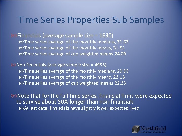
Time Series Properties Sub Samples Financials (average sample size = 1630) Time series average of the monthly medians, 31. 03 Time series average of the monthly means, 31. 51 Time series average of cap weighted means 24. 09 Non Financials (average sample size = 4955) Time series average of the monthly medians, 20. 03 Time series average of the monthly means, 22. 13 Time series average of cap weighted means 22. 23 Note that for the full time series, financial firms were expected to survive about 50% longer than non-financials At last date, financials have slightly lower expected lives

Another Angle on Default Correlations Once the time series of expected lives have been calculated, we can estimate default correlation as the correlation of percentage changes in expected lives across firms As expected lives shorten, changes of a given magnitude become larger percentage changes Since correlation is a bounded function (-1 to +1) larger events drive the correlation values toward the extreme value Two bonds that have one day of expected life each will have a very high default correlation Better than trying to correlate OAS spreads since bond prices are driven by liquidity effects

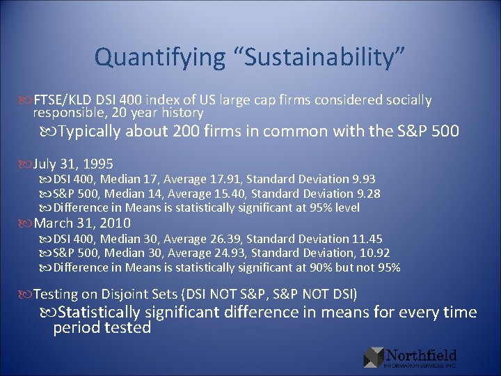
Quantifying “Sustainability” FTSE/KLD DSI 400 index of US large cap firms considered socially responsible, 20 year history Typically about 200 firms in common with the S&P 500 July 31, 1995 DSI 400, Median 17, Average 17. 91, Standard Deviation 9. 93 S&P 500, Median 14, Average 15. 40, Standard Deviation 9. 28 Difference in Means is statistically significant at 95% level March 31, 2010 DSI 400, Median 30, Average 26. 39, Standard Deviation 11. 45 S&P 500, Median 30, Average 24. 93, Standard Deviation, 10. 92 Difference in Means is statistically significant at 90% but not 95% Testing on Disjoint Sets (DSI NOT S&P, S&P NOT DSI) Statistically significant difference in means for every time period tested

A Measure of Systemic Risk? • Obviously, if the market things public companies are not going to be around very long, the economy is in a bad way • Low equity valuations and high leverage equate to short life expectancy – Higher leverage can be sustained with higher growth rates that cause higher equity valuations We propose “revenue weighted” expected average life as a measure of systemic stress on an economy – By revenue weighting we capture the stress in the real economy – Avoids bias of cap weighting since failing firm’s have small market capitalization and don’t count as much • Full sample low values are in the 6 -7 range (1997 -1998) with high value above 30. – From July 2007 to July 2008, went from over 29 to below 12.

Expected Life as a Systemic Risk Measure Full Sample 220 Months N Median Capitalization Weighted Mean Standard Deviation Revenue Weighted Mean All 6587 16. 90 18. 14 8. 05 17. 48 Financials 1631 22. 28 17. 06 16. 80 7. 86 Non. Financials 4955 14. 74 18. 42 7. 79 17. 60

The Equity Factor Risk of a Corporate Bond %Rbt ~ (-(T-B)/B) * (Dp / Dc) * [Sj = 1 to n Bj Fjt] + et] Rbt = the return on bond b during period t T = the value of the bond if it were riskless B = the market value of the bond Dp = the delta of the shareholder put option Dc = the delta of the shareholder call option

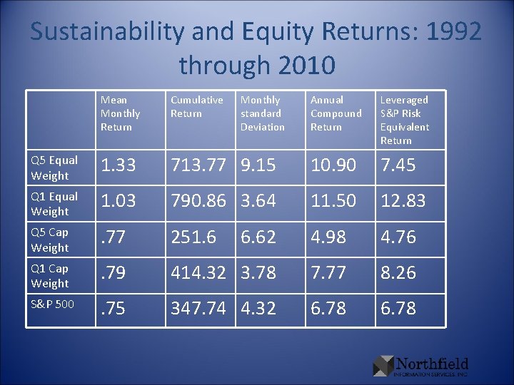
Sustainability and Equity Returns: 1992 through 2010 Mean Monthly Return Cumulative Return Q 5 Equal Weight 1. 33 Q 1 Equal Weight Monthly standard Deviation Annual Compound Return Leveraged S&P Risk Equivalent Return 713. 77 9. 15 10. 90 7. 45 1. 03 790. 86 3. 64 11. 50 12. 83 Q 5 Cap Weight . 77 251. 6 6. 62 4. 98 4. 76 Q 1 Cap Weight . 79 414. 32 3. 78 7. 77 8. 26 S&P 500 . 75 347. 74 4. 32 6. 78

Sustainability and Equity Returns • Portfolio Returns – An equal weighted portfolio of the low sustainability stocks (high risk) in Quintile 5 produced the highest monthly mean return of 1. 33%. The volatility of such this portfolio was so high at over 9% per month that the annualized compound return was only 10. 9%, which is inferior to the 11. 50% annualized compound rate achieved by the equal weighted portfolio of high sustainability (low risk) stocks in Q 1 – It should also be noted that a market capitalization weighted portfolio of high sustainability stocks produce both higher returns and lower risk than the S&P 500. These results ignore trading costs which are apt to be very substantial in the case of equal weighted portfolios – Leveraging up the equal weighted portfolio of high sustainability (low risk) stocks produced nearly a 13% annual compound rate of return, almost double the equivalent risk portfolio of the S&P 500 – For background, see di. Bartolomeo (2007) and Scherer (2010)

Next Steps Use more sophisticated option pricing model that allows for stochastic interest rates and possibly stochastic volatility Use expected life data at the firm level to predict changes in credit ratings We have hand collected (copied from Barron’s week by week) every credit rating down grade and upgrade since 1991 Relate changes in expected life to subsequent rating changes Relate expected life values that are outliers within their rating category to subsequent rating changes Adjust credit risk expectations for bond issuers and financial counterparties in our fixed income risk model

Conclusions Combining factor models and structural models of credit risk allows for consistent estimation of equity risk, credit risk and default correlation Structural models based on contingent claims methods are a direct and informative approach to assessing the expected survival of firms Comparison of SRI and conventional US stock indices reveals a positive and significant difference in expected lives, confirming the existence of “sustainability” Equity return strategies based on our measure of sustainability seem at least as effective as other “low volatility” equity strategies We believe this technology will have usefulness as a measure of systemic risks in developed economies