Equity Investments R 51 Equity Valuation Concepts and

Equity Investments R 51: Equity Valuation: Concepts and Basic Tools

Contents 1. Introduction 2. Estimated Value and Market Price 3. Major Categories of Equity Valuation Models 4. Present Value Models 5. Multiplier Models 6. Asset-Based Valuation 7. Summary and Conclusion Copyright © 2016 All Rights Reserved 2

1. INTRODUCTION Copyright © 2016 All Rights Reserved 3

Introduction Under fundamental analysis, the value of a security is estimated using information about investment fundamentals and characteristics (i. e. GDP growth, industry growth, and quality of and growth in company earnings) and then the estimated value is compared with the market value (price) to make investment decisions. The estimated value is referred to as fundamental value or intrinsic value of a security. Copyright © 2016 All Rights Reserved 4

2. ESTIMATED VALUE AND MARKET PRICE Copyright © 2016 All Rights Reserved 5

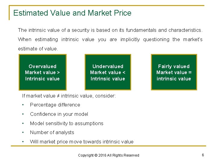
Estimated Value and Market Price The intrinsic value of a security is based on its fundamentals and characteristics. When estimating intrinsic value you are implicitly questioning the market’s estimate of value. Undervalued Market value < Intrinsic value Overvalued Market value > Intrinsic value Fairly valued Market value = intrinsic value If market value ≠ intrinsic value, consider: • Percentage difference • Confidence in your model • Model sensitivity to assumptions • Number of analysts • Will market price move towards intrinsic value Copyright © 2016 All Rights Reserved 6

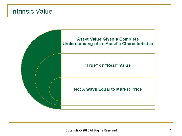
Intrinsic Value Asset Value Given a Complete Understanding of an Asset’s Characteristics “True” or “Real” Value Not Always Equal to Market Price Copyright © 2016 All Rights Reserved 7

3. MAJOR CATEGORIES OF EQUITY VALUATION MODELS Copyright © 2016 All Rights Reserved 8

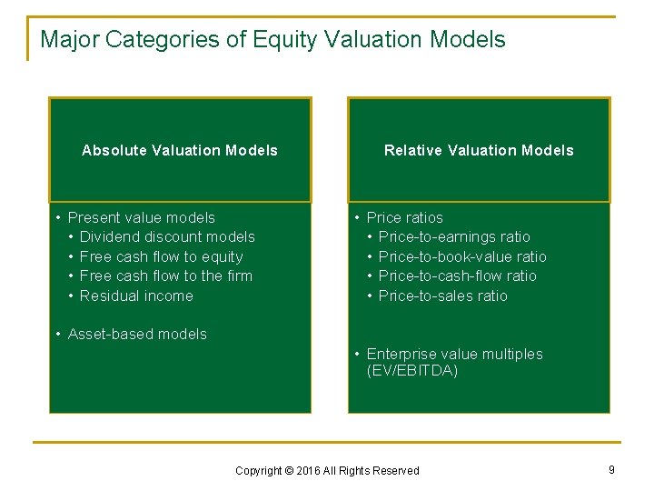
Major Categories of Equity Valuation Models Absolute Valuation Models • Present value models • Dividend discount models • Free cash flow to equity • Free cash flow to the firm • Residual income Relative Valuation Models • Price ratios • Price-to-earnings ratio • Price-to-book-value ratio • Price-to-cash-flow ratio • Price-to-sales ratio • Asset-based models • Enterprise value multiples (EV/EBITDA) Copyright © 2016 All Rights Reserved 9

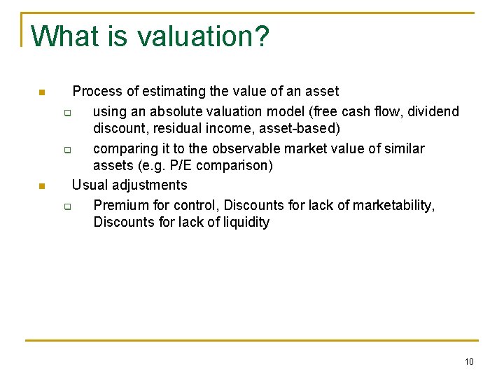
What is valuation? n n Process of estimating the value of an asset q using an absolute valuation model (free cash flow, dividend discount, residual income, asset-based) q comparing it to the observable market value of similar assets (e. g. P/E comparison) Usual adjustments q Premium for control, Discounts for lack of marketability, Discounts for lack of liquidity 10

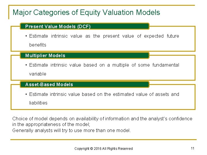
Major Categories of Equity Valuation Models Present Value Models (DCF) • Estimate intrinsic value as the present value of expected future benefits Multiplier Models • Estimate intrinsic value based on a multiple of some fundamental variable Asset-Based Models • Estimate intrinsic value based on the estimated value of assets and liabilities Choice of model depends on availability of information and the analyst’s confidence in the appropriateness of the model; Generally analysts will try to use more than one model. Copyright © 2016 All Rights Reserved 11

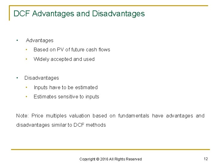
DCF Advantages and Disadvantages • • Advantages • Based on PV of future cash flows • Widely accepted and used Disadvantages • Inputs have to be estimated • Estimates sensitive to inputs Note: Price multiples valuation based on fundamentals have advantages and disadvantages similar to DCF methods Copyright © 2016 All Rights Reserved 12

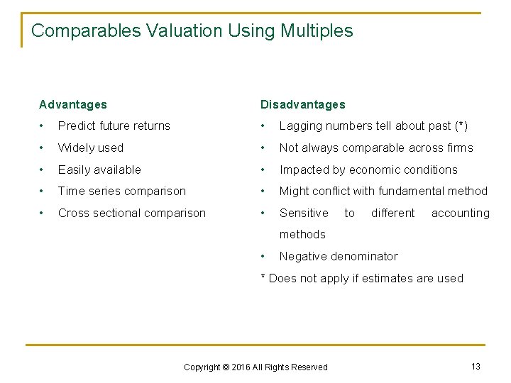
Comparables Valuation Using Multiples Advantages Disadvantages • Predict future returns • Lagging numbers tell about past (*) • Widely used • Not always comparable across firms • Easily available • Impacted by economic conditions • Time series comparison • Might conflict with fundamental method • Cross sectional comparison • Sensitive to different accounting methods • Negative denominator * Does not apply if estimates are used Copyright © 2016 All Rights Reserved 13

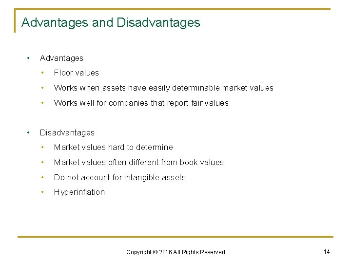
Advantages and Disadvantages • • Advantages • Floor values • Works when assets have easily determinable market values • Works well for companies that report fair values Disadvantages • Market values hard to determine • Market values often different from book values • Do not account for intangible assets • Hyperinflation Copyright © 2016 All Rights Reserved 14

4. PRESENT VALUE MODELS: DIVIDEND DISCOUNT MODEL Copyright © 2016 All Rights Reserved 15

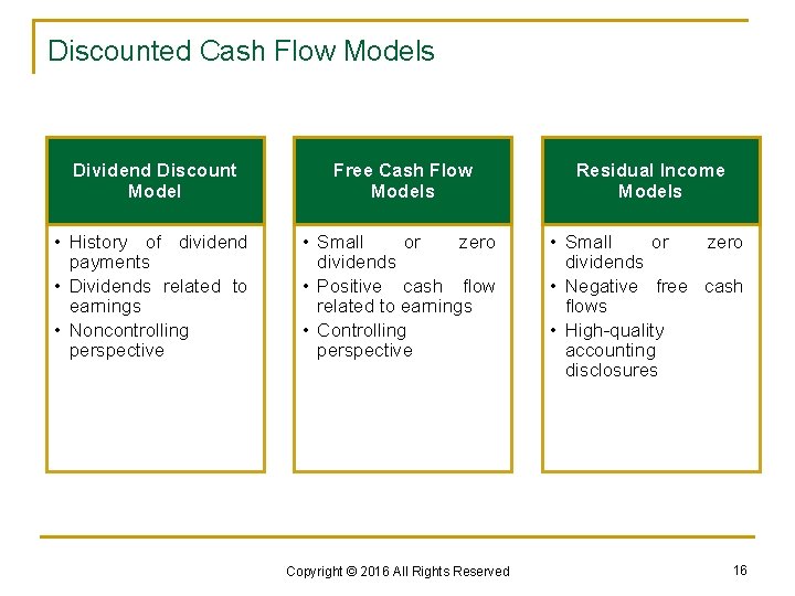
Discounted Cash Flow Models Dividend Discount Model Free Cash Flow Models Residual Income Models • History of dividend payments • Dividends related to earnings • Noncontrolling perspective • Small or zero dividends • Positive cash flow related to earnings • Controlling perspective • Small or zero dividends • Negative free cash flows • High-quality accounting disclosures Copyright © 2016 All Rights Reserved 16

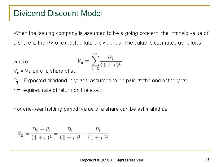
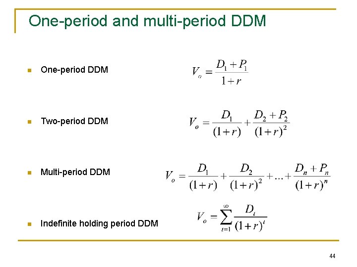
Dividend Discount Model When the issuing company is assumed to be a going concern, the intrinsic value of a share is the PV of expected future dividends. The value is estimated as follows: where, V 0 = Value of a share of stock today, at t = 0 Dt = Expected dividend in year t, assumed to be paid at the end of the year r = required rate of return on the stock For one-year holding period, value of a share can be estimated as: Copyright © 2016 All Rights Reserved 17

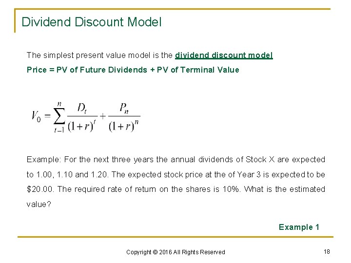
Dividend Discount Model The simplest present value model is the dividend discount model Price = PV of Future Dividends + PV of Terminal Value Example: For the next three years the annual dividends of Stock X are expected to 1. 00, 1. 10 and 1. 20. The expected stock price at the of Year 3 is expected to be $20. 00. The required rate of return on the shares is 10%. What is the estimated value? Example 1 Copyright © 2016 All Rights Reserved 18

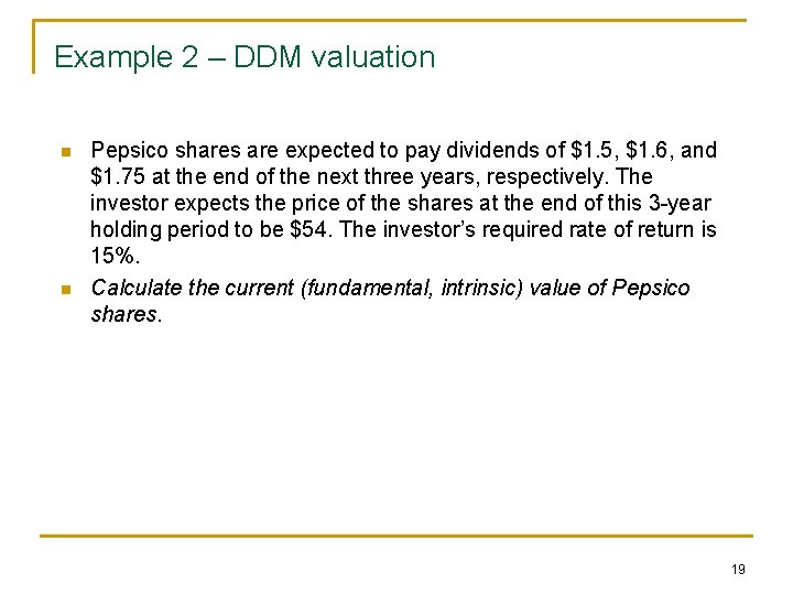
Example 2 – DDM valuation n n Pepsico shares are expected to pay dividends of $1. 5, $1. 6, and $1. 75 at the end of the next three years, respectively. The investor expects the price of the shares at the end of this 3 -year holding period to be $54. The investor’s required rate of return is 15%. Calculate the current (fundamental, intrinsic) value of Pepsico shares. 19

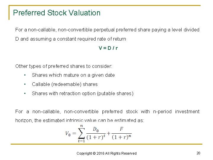
Preferred Stock Valuation For a non-callable, non-convertible perpetual preferred share paying a level divided D and assuming a constant required rate of return V=D/r Other types of preferred shares to consider: • Shares which mature on a given date • Callable (redeemable) shares • Shares with retraction option (putable shares) For a non-callable, non-convertible preferred stock with n-period investment horizon, the estimated intrinsic value can be estimated as: Copyright © 2016 All Rights Reserved 20

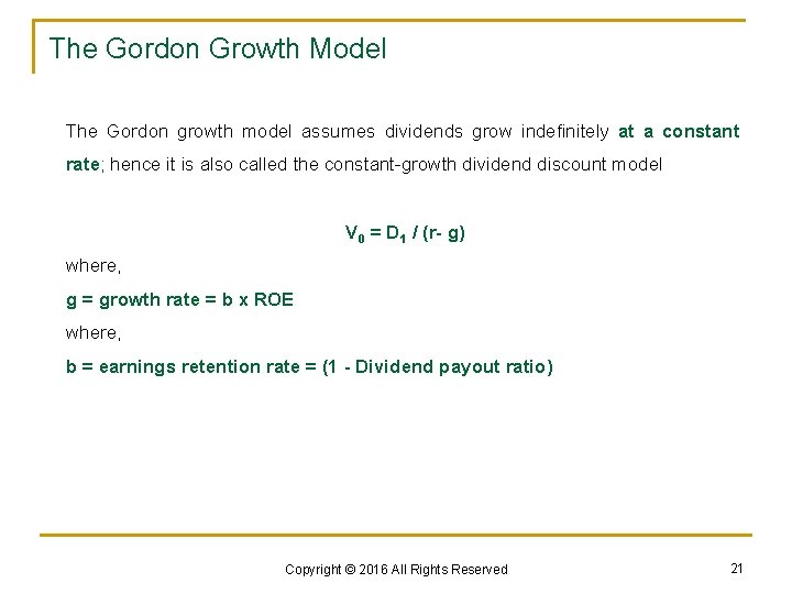
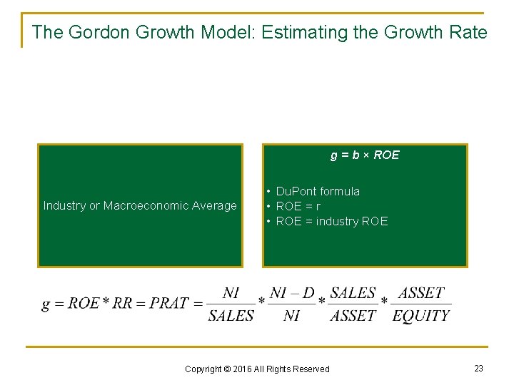
The Gordon Growth Model The Gordon growth model assumes dividends grow indefinitely at a constant rate; hence it is also called the constant-growth dividend discount model V 0 = D 1 / (r- g) where, g = growth rate = b x ROE where, b = earnings retention rate = (1 - Dividend payout ratio) Copyright © 2016 All Rights Reserved 21

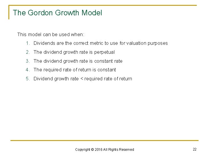
The Gordon Growth Model This model can be used when: 1. Dividends are the correct metric to use for valuation purposes 2. The dividend growth rate is perpetual 3. The dividend growth rate is constant rate 4. The required rate of return is constant 5. Dividend growth rate < required rate of return Copyright © 2016 All Rights Reserved 22

The Gordon Growth Model: Estimating the Growth Rate g = b × ROE Industry or Macroeconomic Average • Du. Pont formula • ROE = r • ROE = industry ROE Copyright © 2016 All Rights Reserved 23

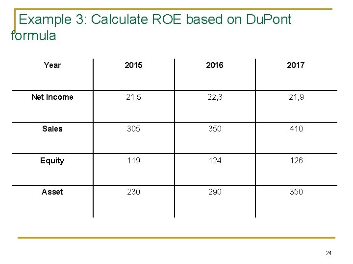
Example 3: Calculate ROE based on Du. Pont formula Year 2015 2016 2017 Net Income 21, 5 22, 3 21, 9 Sales 305 350 410 Equity 119 124 126 Asset 230 290 350 24

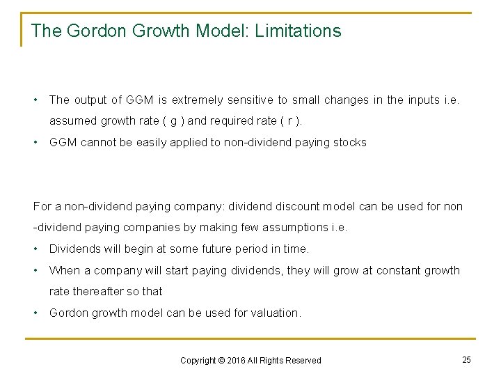
The Gordon Growth Model: Limitations • The output of GGM is extremely sensitive to small changes in the inputs i. e. assumed growth rate ( g ) and required rate ( r ). • GGM cannot be easily applied to non-dividend paying stocks For a non-dividend paying company: dividend discount model can be used for non -dividend paying companies by making few assumptions i. e. • Dividends will begin at some future period in time. • When a company will start paying dividends, they will grow at constant growth rate thereafter so that • Gordon growth model can be used for valuation. Copyright © 2016 All Rights Reserved 25

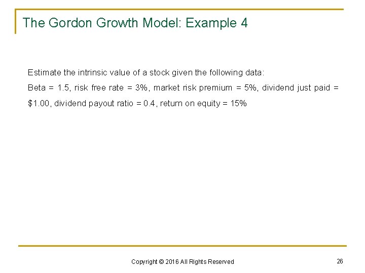
The Gordon Growth Model: Example 4 Estimate the intrinsic value of a stock given the following data: Beta = 1. 5, risk free rate = 3%, market risk premium = 5%, dividend just paid = $1. 00, dividend payout ratio = 0. 4, return on equity = 15% Copyright © 2016 All Rights Reserved 26

The Gordon Growth Model: Example 5 (No Current DIV) A company does not currently pay dividend but is expected to begin to do so in 4 years. The first dividend is expected to be $2. 00 and to be received at the end of Year 4. The dividend is expected to grow at 5% into perpetuity. The required return is 10%. What is the estimated current intrinsic value? Example 7 Copyright © 2016 All Rights Reserved 27

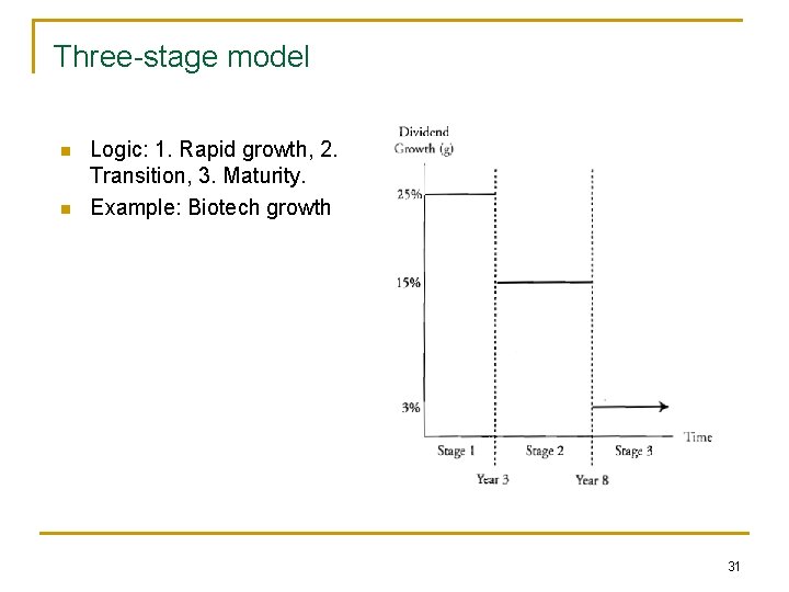
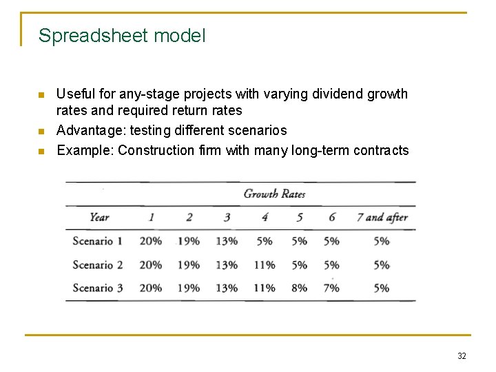
Multistage growth models In the case that dividend growth varies over time we need to use multistage growth models The required rate of return applicable to each stage might also be different (depends on a phase riskiness; e. g. supernormal growth stage will have higher risk and higher required rate of return) Four generic types of multistage models: n n n 1. 2. 3. 4. Two-stage H-model (will be covered in Level 2) Three-stage Spreadsheet model 28

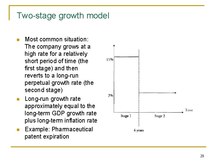
Two-stage growth model n n n Most common situation: The company grows at a high rate for a relatively short period of time (the first stage) and then reverts to a long-run perpetual growth rate (the second stage) Long-run growth rate approximately equal to the long-term GDP growth rate plus long-term inflation rate Example: Pharmaceutical patent expiration 29

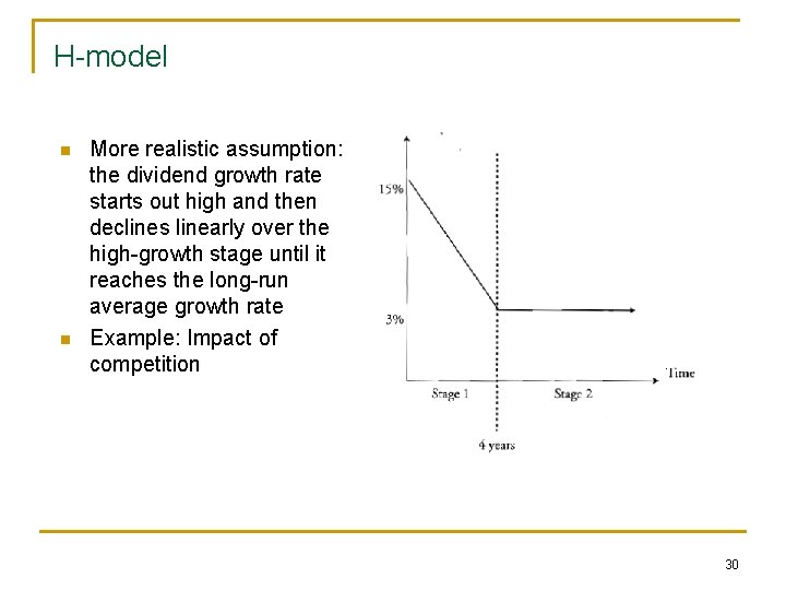
H-model n n More realistic assumption: the dividend growth rate starts out high and then declines linearly over the high-growth stage until it reaches the long-run average growth rate Example: Impact of competition 30

Three-stage model n n Logic: 1. Rapid growth, 2. Transition, 3. Maturity. Example: Biotech growth 31

Spreadsheet model n n n Useful for any-stage projects with varying dividend growth rates and required return rates Advantage: testing different scenarios Example: Construction firm with many long-term contracts 32

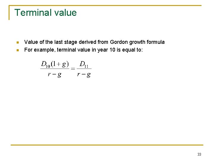
Terminal value n n Value of the last stage derived from Gordon growth formula For example, terminal value in year 10 is equal to: 33

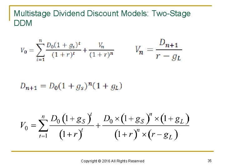
Multistage Dividend Discount Models: Two-Stage DDM • Multistage growth models assume that dividends grow at different growth rates rather than constant growth rate. • They are most appropriate to use for rapidly growing companies. Two-stage DDM: In this model, dividends are expected to grow at two growth rates over time i. e. 1. Stage 1 represents abnormal growth i. e. high growth rate for an initial, finite period of time i. e. for n years. It is represented by g. S (short-term growth rate). 2. Stage 2 represents lower, sustainable growth rate for an indefinite period. It is represented by g. L(long-term growth rate). Copyright © 2016 All Rights Reserved 34

Multistage Dividend Discount Models: Two-Stage DDM Copyright © 2016 All Rights Reserved 35

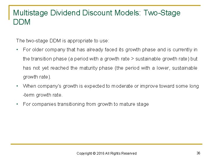
Multistage Dividend Discount Models: Two-Stage DDM The two-stage DDM is appropriate to use: • For older company that has already faced its growth phase and is currently in the transition phase (a period with a growth rate > sustainable growth rate) but has not yet reached the maturity phase (the period with a lower, sustainable growth rate). • When company’s growth is expected to moderate or improve toward some long -term growth rate. • For companies transitioning from growth to mature stage Copyright © 2016 All Rights Reserved 36

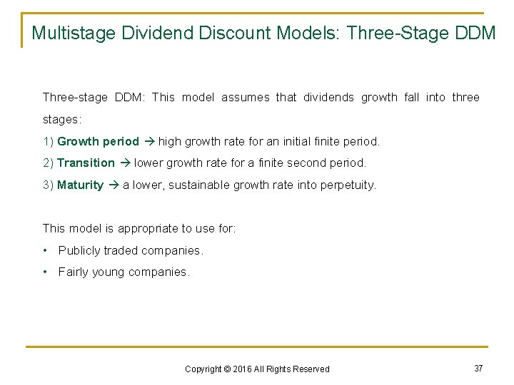
Multistage Dividend Discount Models: Three-Stage DDM Three-stage DDM: This model assumes that dividends growth fall into three stages: 1) Growth period high growth rate for an initial finite period. 2) Transition lower growth rate for a finite second period. 3) Maturity a lower, sustainable growth rate into perpetuity. This model is appropriate to use for: • Publicly traded companies. • Fairly young companies. Copyright © 2016 All Rights Reserved 37

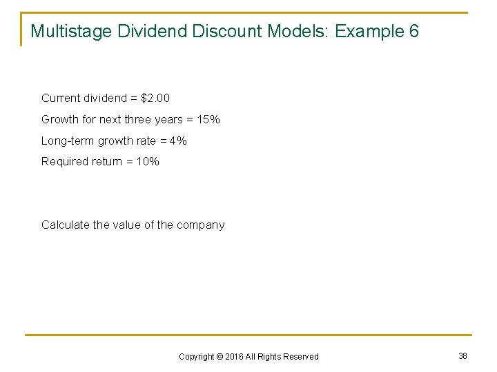
Multistage Dividend Discount Models: Example 6 Current dividend = $2. 00 Growth for next three years = 15% Long-term growth rate = 4% Required return = 10% Calculate the value of the company Copyright © 2016 All Rights Reserved 38

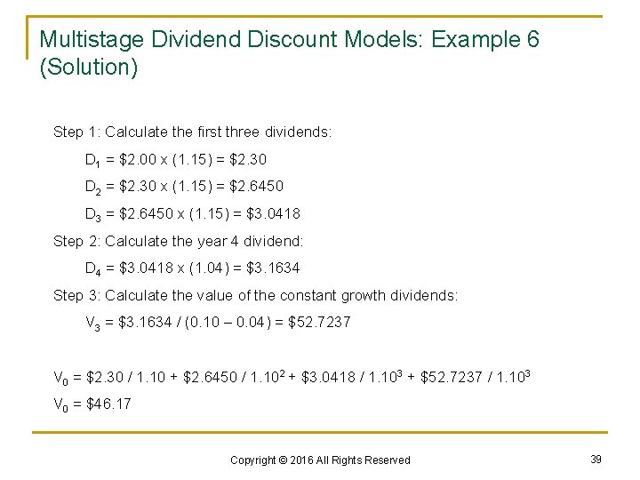
Multistage Dividend Discount Models: Example 6 (Solution) Step 1: Calculate the first three dividends: D 1 = $2. 00 x (1. 15) = $2. 30 D 2 = $2. 30 x (1. 15) = $2. 6450 D 3 = $2. 6450 x (1. 15) = $3. 0418 Step 2: Calculate the year 4 dividend: D 4 = $3. 0418 x (1. 04) = $3. 1634 Step 3: Calculate the value of the constant growth dividends: V 3 = $3. 1634 / (0. 10 – 0. 04) = $52. 7237 V 0 = $2. 30 / 1. 10 + $2. 6450 / 1. 102 + $3. 0418 / 1. 103 + $52. 7237 / 1. 103 V 0 = $46. 17 Copyright © 2016 All Rights Reserved 39

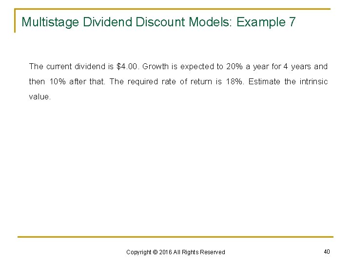
Multistage Dividend Discount Models: Example 7 The current dividend is $4. 00. Growth is expected to 20% a year for 4 years and then 10% after that. The required rate of return is 18%. Estimate the intrinsic value. Copyright © 2016 All Rights Reserved 40

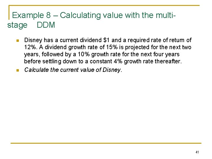
Example 8 – Calculating value with the multistage DDM n n Disney has a current dividend $1 and a required rate of return of 12%. A dividend growth rate of 15% is projected for the next two years, followed by a 10% growth rate for the next four years before settling down to a constant 4% growth rate thereafter. Calculate the current value of Disney. 41

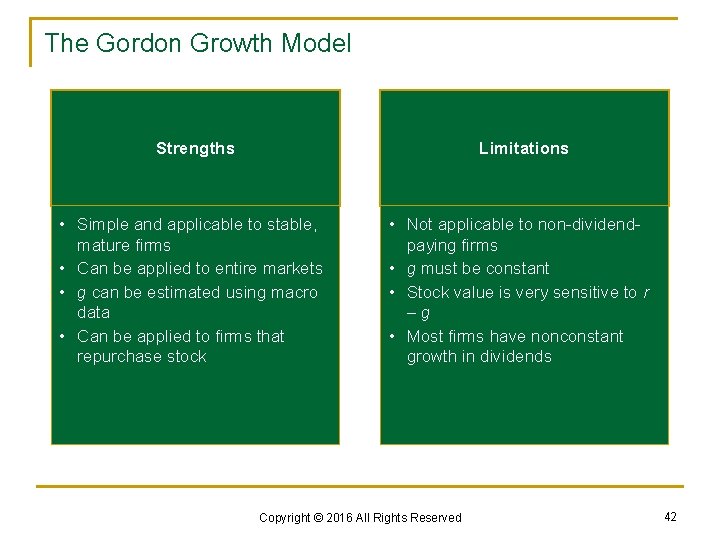
The Gordon Growth Model Strengths Limitations • Simple and applicable to stable, mature firms • Can be applied to entire markets • g can be estimated using macro data • Can be applied to firms that repurchase stock • Not applicable to non-dividendpaying firms • g must be constant • Stock value is very sensitive to r –g • Most firms have nonconstant growth in dividends Copyright © 2016 All Rights Reserved 42

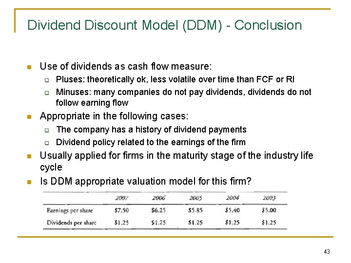
Dividend Discount Model (DDM) - Conclusion n Use of dividends as cash flow measure: q q n Appropriate in the following cases: q q n n Pluses: theoretically ok, less volatile over time than FCF or RI Minuses: many companies do not pay dividends, dividends do not follow earning flow The company has a history of dividend payments Dividend policy related to the earnings of the firm Usually applied for firms in the maturity stage of the industry life cycle Is DDM appropriate valuation model for this firm? 43

One-period and multi-period DDM n One-period DDM n Two-period DDM n Multi-period DDM n Indefinite holding period DDM 44

FREE CASH FLOW MODEL Copyright © 2016 All Rights Reserved 45

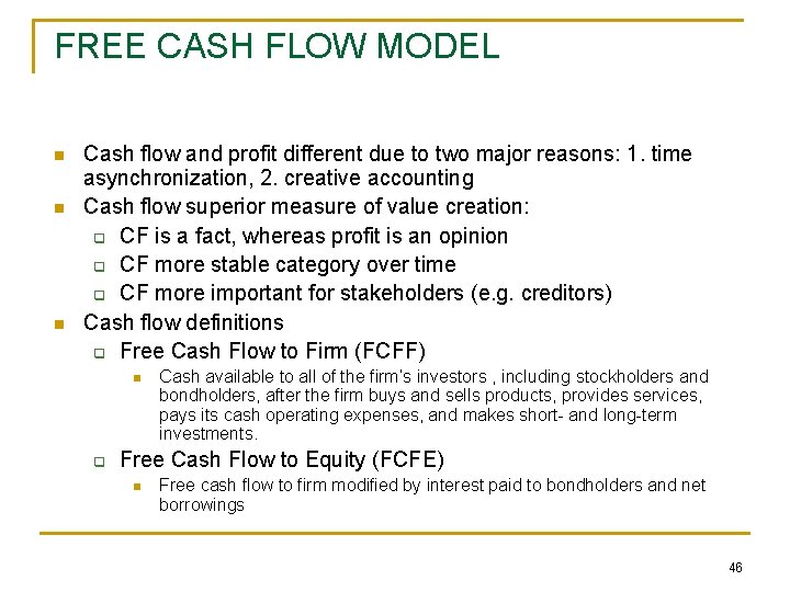
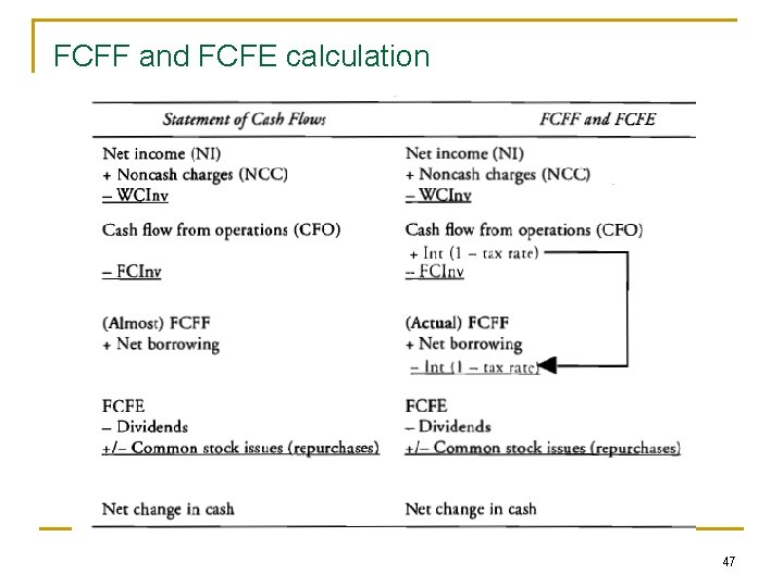
FREE CASH FLOW MODEL n n n Cash flow and profit different due to two major reasons: 1. time asynchronization, 2. creative accounting Cash flow superior measure of value creation: q CF is a fact, whereas profit is an opinion q CF more stable category over time q CF more important for stakeholders (e. g. creditors) Cash flow definitions q Free Cash Flow to Firm (FCFF) n q Cash available to all of the firm’s investors , including stockholders and bondholders, after the firm buys and sells products, provides services, pays its cash operating expenses, and makes short- and long-term investments. Free Cash Flow to Equity (FCFE) n Free cash flow to firm modified by interest paid to bondholders and net borrowings 46

FCFF and FCFE calculation 47

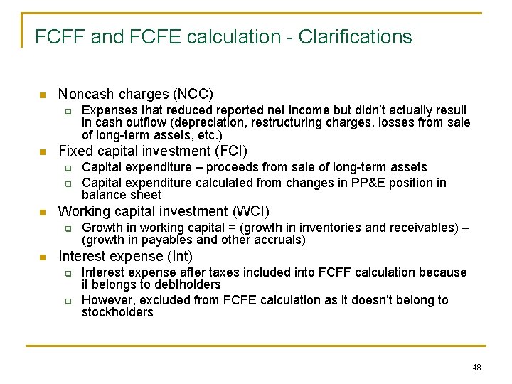
FCFF and FCFE calculation - Clarifications n Noncash charges (NCC) q n Fixed capital investment (FCI) q q n Capital expenditure – proceeds from sale of long-term assets Capital expenditure calculated from changes in PP&E position in balance sheet Working capital investment (WCI) q n Expenses that reduced reported net income but didn’t actually result in cash outflow (depreciation, restructuring charges, losses from sale of long-term assets, etc. ) Growth in working capital = (growth in inventories and receivables) – (growth in payables and other accruals) Interest expense (Int) q q Interest expense after taxes included into FCFF calculation because it belongs to debtholders However, excluded from FCFE calculation as it doesn’t belong to stockholders 48

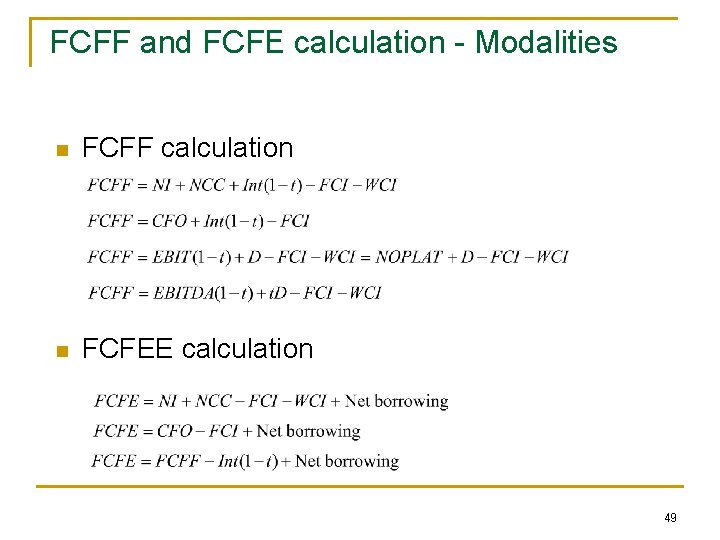
FCFF and FCFE calculation - Modalities n FCFF calculation n FCFEE calculation 49

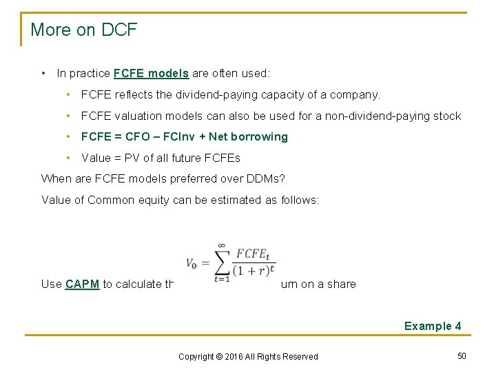
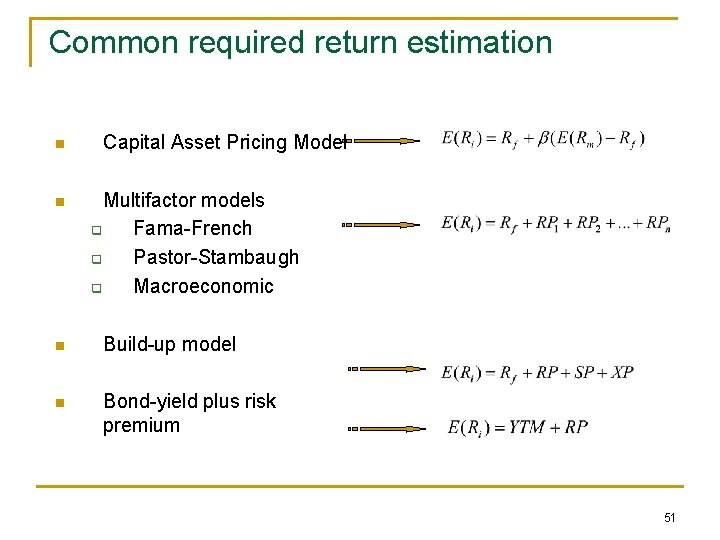
More on DCF • In practice FCFE models are often used: • FCFE reflects the dividend-paying capacity of a company. • FCFE valuation models can also be used for a non-dividend-paying stock • FCFE = CFO – FCInv + Net borrowing • Value = PV of all future FCFEs When are FCFE models preferred over DDMs? Value of Common equity can be estimated as follows: Use CAPM to calculate the required rate of return on a share Example 4 Copyright © 2016 All Rights Reserved 50

Common required return estimation n n Capital Asset Pricing Model Multifactor models q Fama-French q Pastor-Stambaugh q Macroeconomic n Build-up model n Bond-yield plus risk premium 51

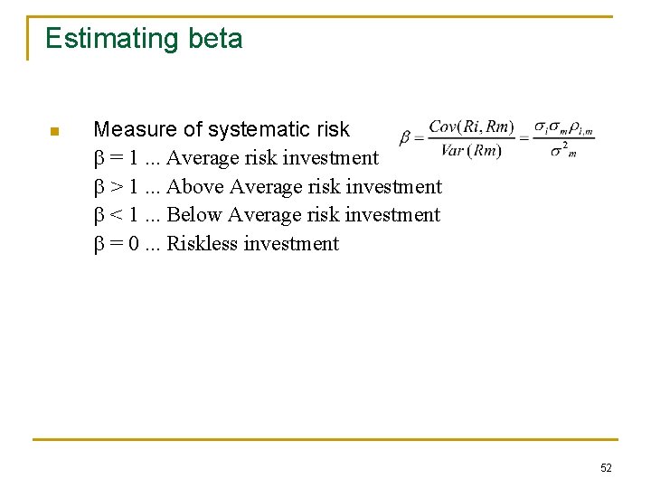
Estimating beta n Measure of systematic risk b = 1. . . Average risk investment b > 1. . . Above Average risk investment b < 1. . . Below Average risk investment b = 0. . . Riskless investment 52

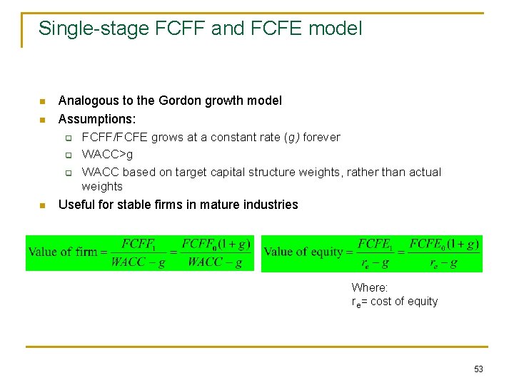
Single-stage FCFF and FCFE model n n Analogous to the Gordon growth model Assumptions: q q q n FCFF/FCFE grows at a constant rate (g) forever WACC>g WACC based on target capital structure weights, rather than actual weights Useful for stable firms in mature industries Where: r e= cost of equity 53

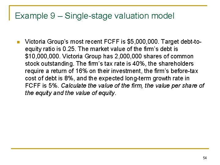
Example 9 – Single-stage valuation model n Victoria Group’s most recent FCFF is $5, 000. Target debt-toequity ratio is 0. 25. The market value of the firm’s debt is $10, 000. Victoria Group has 2, 000 shares of common stock outstanding. The firm’s tax rate is 40%, the shareholders require a return of 16% on their investment, the firm’s before-tax cost of debt is 8%, and the expected long-term growth rate in FCFF is 5%. Calculate the value of the firm, the value per share of the equity and the value of equity. 54

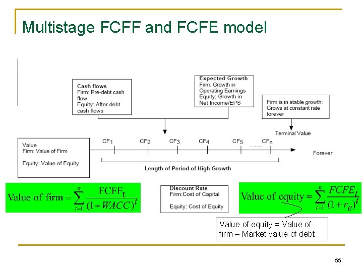
Multistage FCFF and FCFE model Value of equity = Value of firm – Market value of debt 55

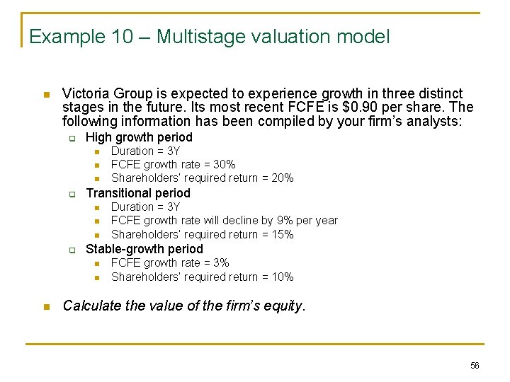
Example 10 – Multistage valuation model n Victoria Group is expected to experience growth in three distinct stages in the future. Its most recent FCFE is $0. 90 per share. The following information has been compiled by your firm’s analysts: q High growth period n n n q Transitional period n n n q Duration = 3 Y FCFE growth rate will decline by 9% per year Shareholders’ required return = 15% Stable-growth period n n n Duration = 3 Y FCFE growth rate = 30% Shareholders’ required return = 20% FCFE growth rate = 3% Shareholders’ required return = 10% Calculate the value of the firm’s equity. 56

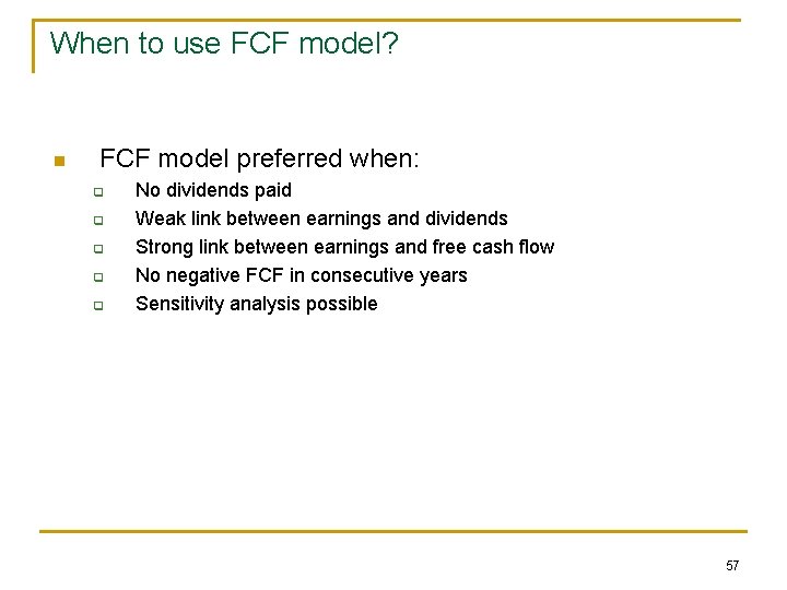
When to use FCF model? n FCF model preferred when: q q q No dividends paid Weak link between earnings and dividends Strong link between earnings and free cash flow No negative FCF in consecutive years Sensitivity analysis possible 57

MULTIPLIER MODEL Copyright © 2016 All Rights Reserved 58

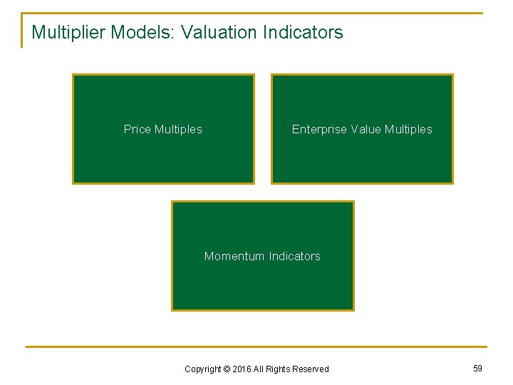
Multiplier Models: Valuation Indicators Price Multiples Enterprise Value Multiples Momentum Indicators Copyright © 2016 All Rights Reserved 59

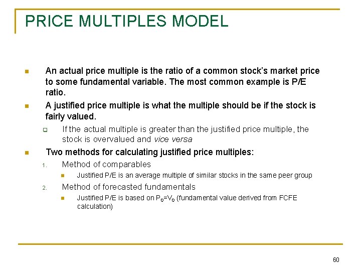
PRICE MULTIPLES MODEL n n An actual price multiple is the ratio of a common stock’s market price to some fundamental variable. The most common example is P/E ratio. A justified price multiple is what the multiple should be if the stock is fairly valued. q n If the actual multiple is greater than the justified price multiple, the stock is overvalued and vice versa Two methods for calculating justified price multiples: 1. Method of comparables n 2. Justified P/E is an average multiple of similar stocks in the same peer group Method of forecasted fundamentals n Justified P/E is based on P 0=V 0 (fundamental value derived from FCFE calculation) 60

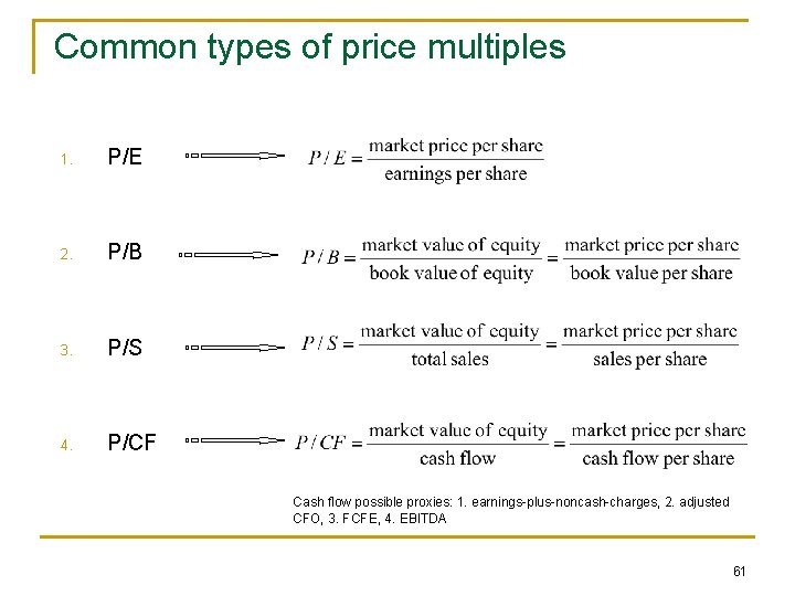
Common types of price multiples 1. P/E 2. P/B 3. P/S 4. P/CF Cash flow possible proxies: 1. earnings-plus-noncash-charges, 2. adjusted CFO, 3. FCFE, 4. EBITDA 61

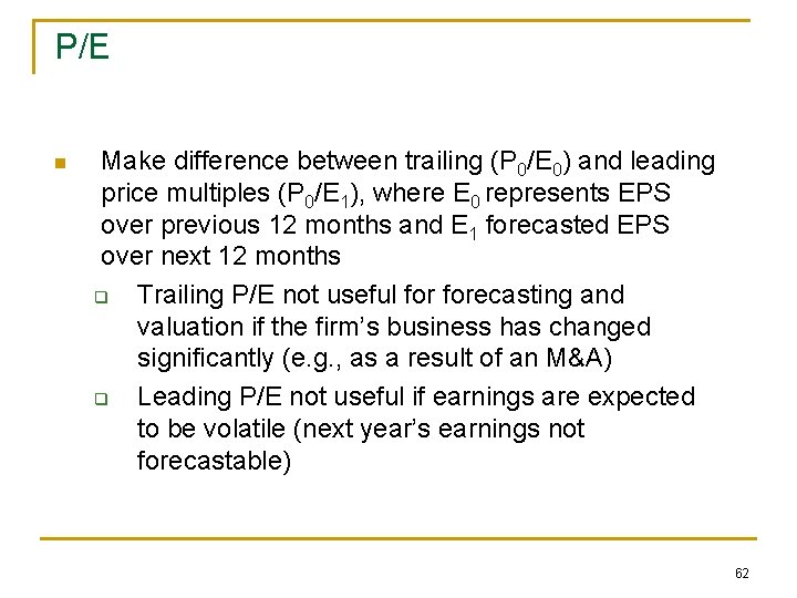
P/E n Make difference between trailing (P 0/E 0) and leading price multiples (P 0/E 1), where E 0 represents EPS over previous 12 months and E 1 forecasted EPS over next 12 months q Trailing P/E not useful forecasting and valuation if the firm’s business has changed significantly (e. g. , as a result of an M&A) q Leading P/E not useful if earnings are expected to be volatile (next year’s earnings not forecastable) 62

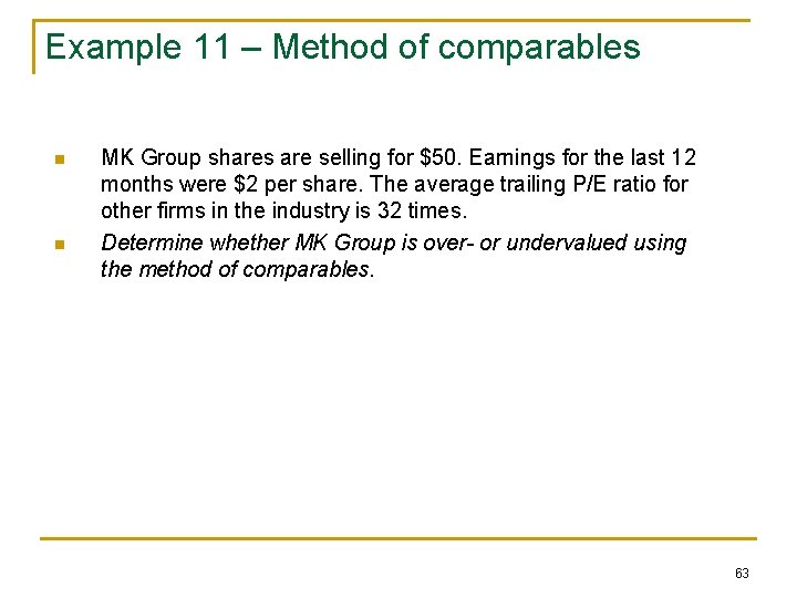
Example 11 – Method of comparables n n MK Group shares are selling for $50. Earnings for the last 12 months were $2 per share. The average trailing P/E ratio for other firms in the industry is 32 times. Determine whether MK Group is over- or undervalued using the method of comparables. 63

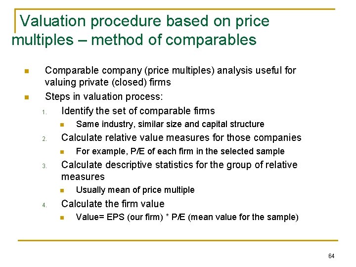
Valuation procedure based on price multiples – method of comparables n n Comparable company (price multiples) analysis useful for valuing private (closed) firms Steps in valuation process: 1. Identify the set of comparable firms n 2. Calculate relative value measures for those companies n 3. For example, P/E of each firm in the selected sample Calculate descriptive statistics for the group of relative measures n 4. Same industry, similar size and capital structure Usually mean of price multiple Calculate the firm value n Value= EPS (our firm) * P/E (mean value for the sample) 64

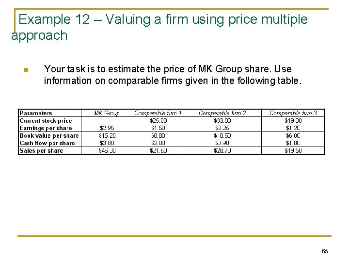
Example 12 – Valuing a firm using price multiple approach n Your task is to estimate the price of MK Group share. Use information on comparable firms given in the following table. 65

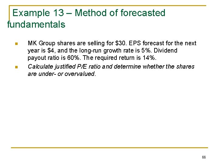
Example 13 – Method of forecasted fundamentals n n MK Group shares are selling for $30. EPS forecast for the next year is $4, and the long-run growth rate is 5%. Dividend payout ratio is 60%. The required return is 14%. Calculate justified P/E ratio and determine whether the shares are under- or overvalued. 66

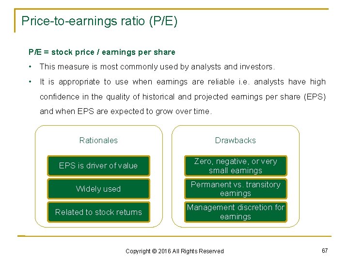
Price-to-earnings ratio (P/E) P/E = stock price / earnings per share • This measure is most commonly used by analysts and investors. • It is appropriate to use when earnings are reliable i. e. analysts have high confidence in the quality of historical and projected earnings per share (EPS) and when EPS are expected to grow over time. Rationales Drawbacks EPS is driver of value Zero, negative, or very small earnings Widely used Permanent vs. transitory earnings Related to stock returns Management discretion for earnings Copyright © 2016 All Rights Reserved 67

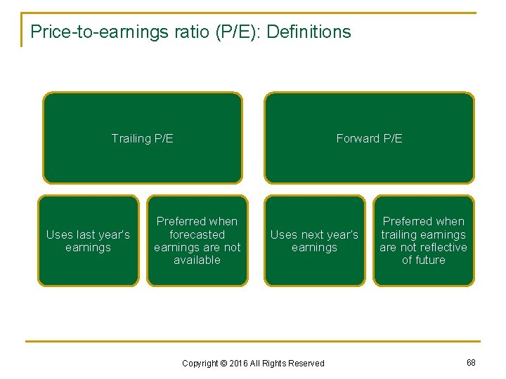
Price-to-earnings ratio (P/E): Definitions Trailing P/E Uses last year’s earnings Forward P/E Preferred when forecasted earnings are not available Uses next year’s earnings Copyright © 2016 All Rights Reserved Preferred when trailing earnings are not reflective of future 68

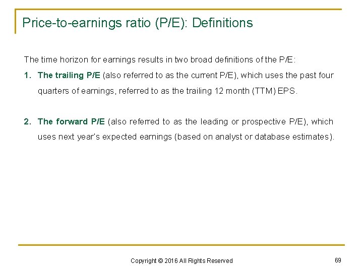
Price-to-earnings ratio (P/E): Definitions The time horizon for earnings results in two broad definitions of the P/E: 1. The trailing P/E (also referred to as the current P/E), which uses the past four quarters of earnings, referred to as the trailing 12 month (TTM) EPS. 2. The forward P/E (also referred to as the leading or prospective P/E), which uses next year’s expected earnings (based on analyst or database estimates). Copyright © 2016 All Rights Reserved 69

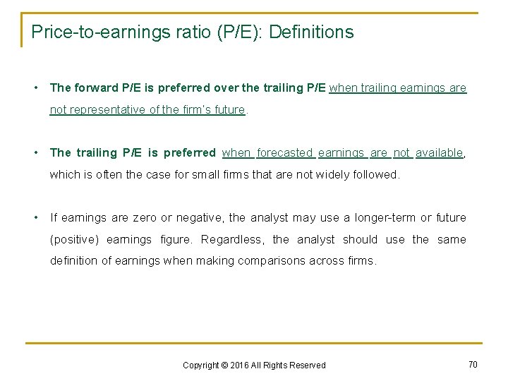
Price-to-earnings ratio (P/E): Definitions • The forward P/E is preferred over the trailing P/E when trailing earnings are not representative of the firm’s future. • The trailing P/E is preferred when forecasted earnings are not available, which is often the case for small firms that are not widely followed. • If earnings are zero or negative, the analyst may use a longer-term or future (positive) earnings figure. Regardless, the analyst should use the same definition of earnings when making comparisons across firms. Copyright © 2016 All Rights Reserved 70

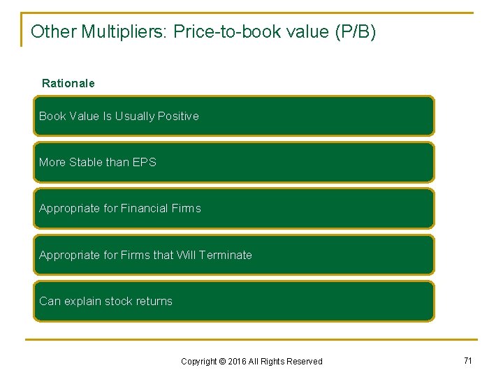
Other Multipliers: Price-to-book value (P/B) Rationale Book Value Is Usually Positive More Stable than EPS Appropriate for Financial Firms Appropriate for Firms that Will Terminate Can explain stock returns Copyright © 2016 All Rights Reserved 71

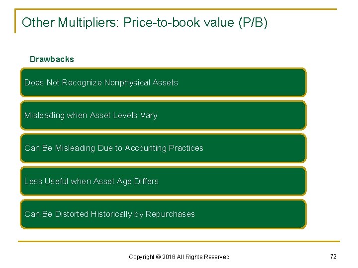
Other Multipliers: Price-to-book value (P/B) Drawbacks Does Not Recognize Nonphysical Assets Misleading when Asset Levels Vary Can Be Misleading Due to Accounting Practices Less Useful when Asset Age Differs Can Be Distorted Historically by Repurchases Copyright © 2016 All Rights Reserved 72

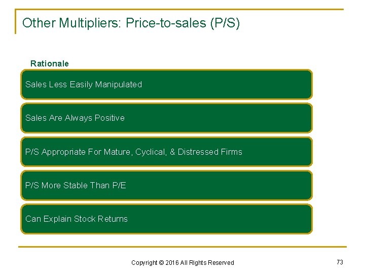
Other Multipliers: Price-to-sales (P/S) Rationale Sales Less Easily Manipulated Sales Are Always Positive P/S Appropriate For Mature, Cyclical, & Distressed Firms P/S More Stable Than P/E Can Explain Stock Returns Copyright © 2016 All Rights Reserved 73

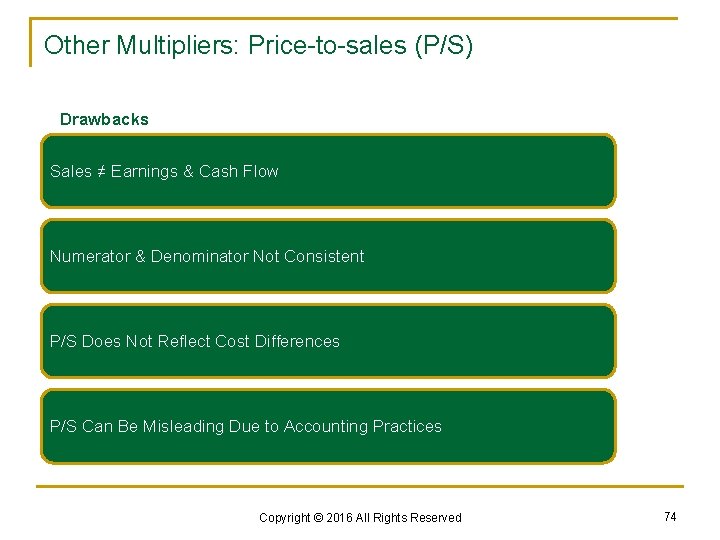
Other Multipliers: Price-to-sales (P/S) Drawbacks Sales ≠ Earnings & Cash Flow Numerator & Denominator Not Consistent P/S Does Not Reflect Cost Differences P/S Can Be Misleading Due to Accounting Practices Copyright © 2016 All Rights Reserved 74

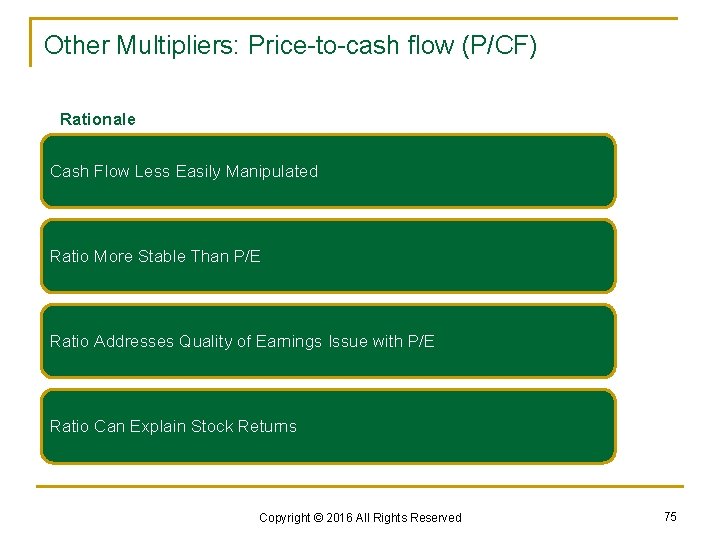
Other Multipliers: Price-to-cash flow (P/CF) Rationale Cash Flow Less Easily Manipulated Ratio More Stable Than P/E Ratio Addresses Quality of Earnings Issue with P/E Ratio Can Explain Stock Returns Copyright © 2016 All Rights Reserved 75

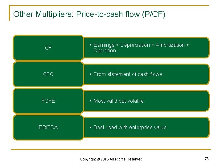
Other Multipliers: Price-to-cash flow (P/CF) CF • Earnings + Depreciation + Amortization + Depletion CFO • From statement of cash flows FCFE • Most valid but volatile EBITDA • Best used with enterprise value Copyright © 2016 All Rights Reserved 76

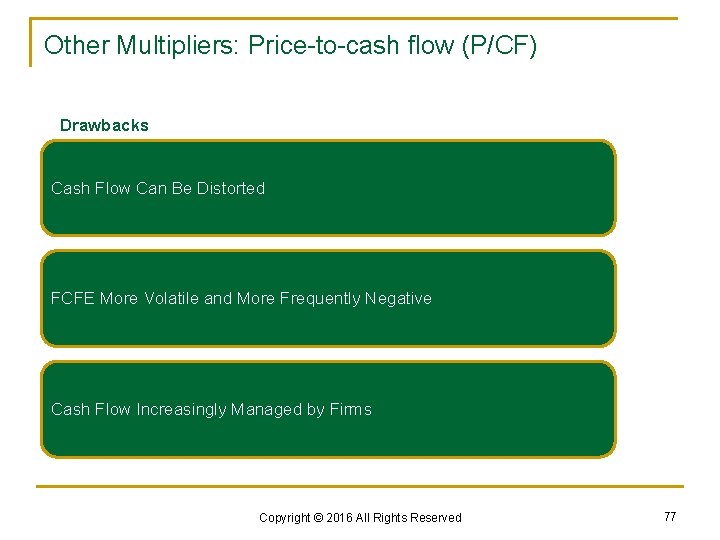
Other Multipliers: Price-to-cash flow (P/CF) Drawbacks Cash Flow Can Be Distorted FCFE More Volatile and More Frequently Negative Cash Flow Increasingly Managed by Firms Copyright © 2016 All Rights Reserved 77

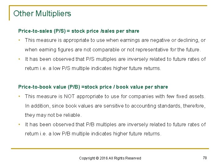
Other Multipliers Price-to-sales (P/S) = stock price /sales per share • This measure is appropriate to use when earnings are negative or declining, or when earning figures are not comparable or not representative for the future. • It has been observed that P/S multiples are inversely related to future rates of return i. e. a low P/S multiple indicates higher future returns. Price-to-book value (P/B) =stock price / book value per share • This measure is NOT appropriate to use for companies with few fixed assets. In addition, since book values are sensitive to accounting standards, therefore, they may not be reliable. • It has been observed that P/B multiples are inversely related to future rates of return i. e. a low P/B multiple indicates higher future returns. Copyright © 2016 All Rights Reserved 78

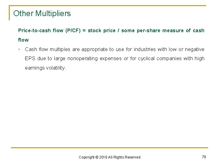
Other Multipliers Price-to-cash flow (P/CF) = stock price / some per-share measure of cash flow • Cash flow multiples are appropriate to use for industries with low or negative EPS due to large nonoperating expenses or for cyclical companies with high earnings volatility. Copyright © 2016 All Rights Reserved 79

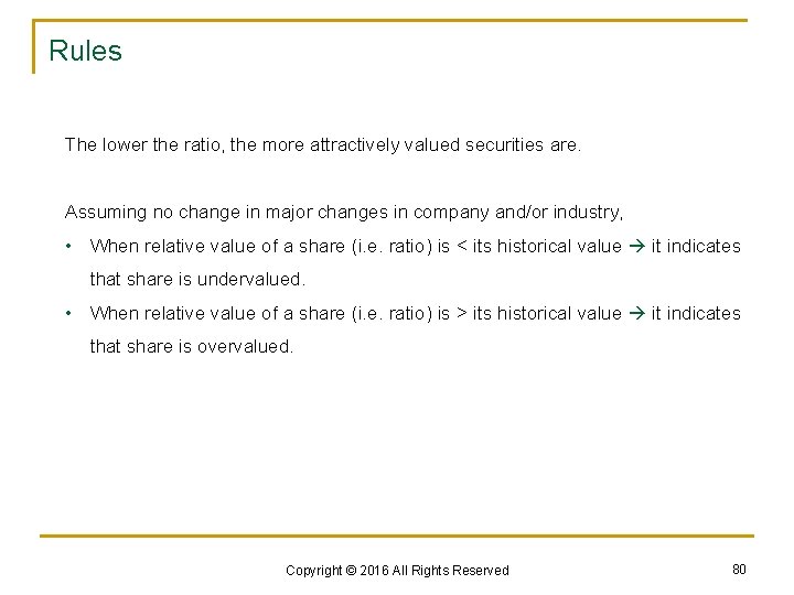
Rules The lower the ratio, the more attractively valued securities are. Assuming no change in major changes in company and/or industry, • When relative value of a share (i. e. ratio) is < its historical value it indicates that share is undervalued. • When relative value of a share (i. e. ratio) is > its historical value it indicates that share is overvalued. Copyright © 2016 All Rights Reserved 80

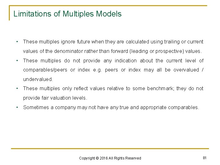
Limitations of Multiples Models • These multiples ignore future when they are calculated using trailing or current values of the denominator rather than forward (leading or prospective) values. • These multiples do not provide any indication about the current level of comparables/peers or index e. g. peers or index may all be overvalued / undervalued. • These multiples only reflect values relative to some benchmark; they do not provide fair valuation levels. • Sometimes a company may not have any true and appropriate comparables. Copyright © 2016 All Rights Reserved 81

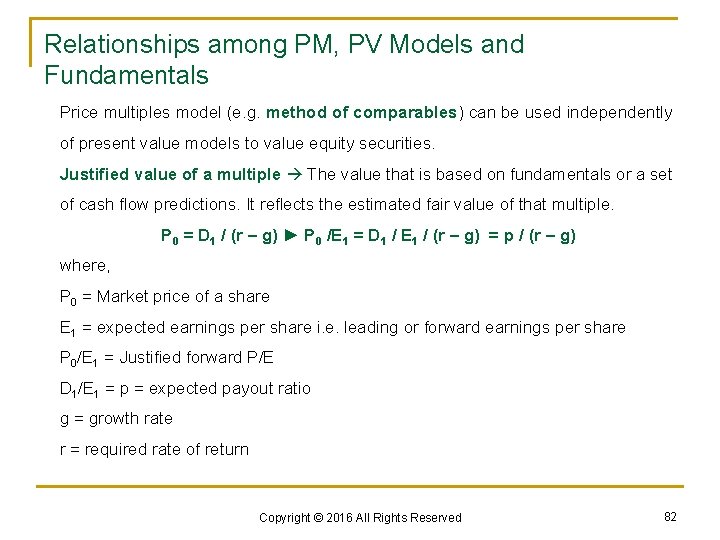
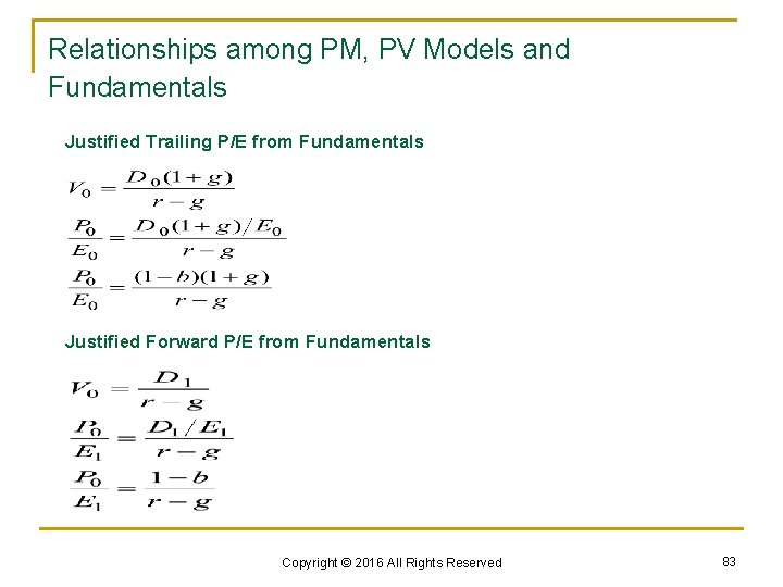
Relationships among PM, PV Models and Fundamentals Price multiples model (e. g. method of comparables) can be used independently of present value models to value equity securities. Justified value of a multiple The value that is based on fundamentals or a set of cash flow predictions. It reflects the estimated fair value of that multiple. P 0 = D 1 / (r – g) ► P 0 /E 1 = D 1 / E 1 / (r – g) = p / (r – g) where, P 0 = Market price of a share E 1 = expected earnings per share i. e. leading or forward earnings per share P 0/E 1 = Justified forward P/E D 1/E 1 = p = expected payout ratio g = growth rate r = required rate of return Copyright © 2016 All Rights Reserved 82

Relationships among PM, PV Models and Fundamentals Justified Trailing P/E from Fundamentals Justified Forward P/E from Fundamentals Copyright © 2016 All Rights Reserved 83

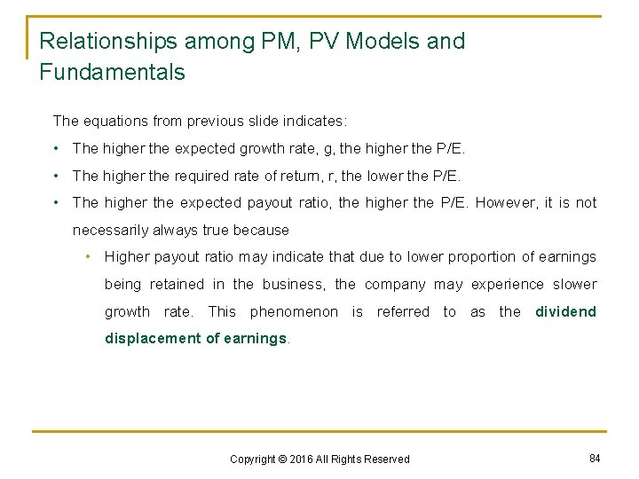
Relationships among PM, PV Models and Fundamentals The equations from previous slide indicates: • The higher the expected growth rate, g, the higher the P/E. • The higher the required rate of return, r, the lower the P/E. • The higher the expected payout ratio, the higher the P/E. However, it is not necessarily always true because • Higher payout ratio may indicate that due to lower proportion of earnings being retained in the business, the company may experience slower growth rate. This phenomenon is referred to as the dividend displacement of earnings. Copyright © 2016 All Rights Reserved 84

Interpretation of P/E ratio The P/E ratio represents how many dollars the investor is willing to pay for a dollar of expected future earnings per share. Note: Justified forward P/E estimates are sensitive to small changes in assumptions. Therefore, it is useful to conduct a sensitivity analysis. Copyright © 2016 All Rights Reserved 85

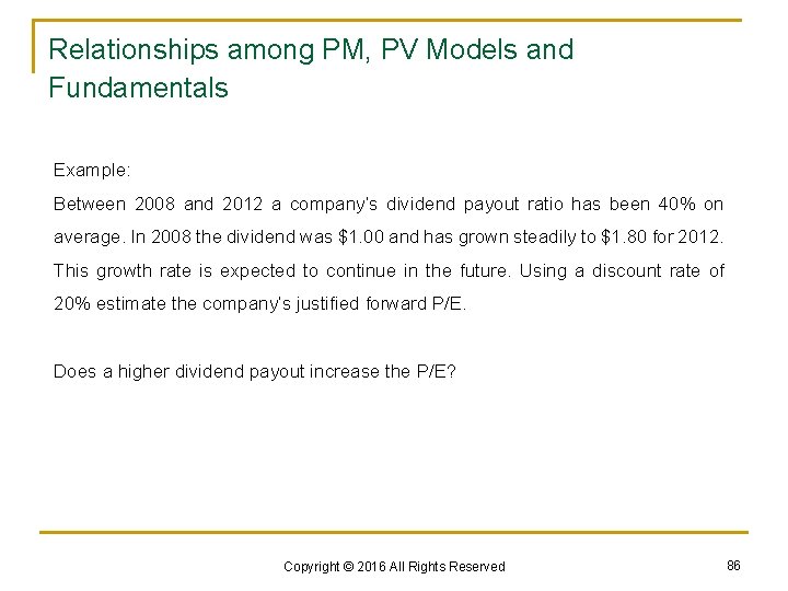
Relationships among PM, PV Models and Fundamentals Example: Between 2008 and 2012 a company’s dividend payout ratio has been 40% on average. In 2008 the dividend was $1. 00 and has grown steadily to $1. 80 for 2012. This growth rate is expected to continue in the future. Using a discount rate of 20% estimate the company’s justified forward P/E. Does a higher dividend payout increase the P/E? Copyright © 2016 All Rights Reserved 86

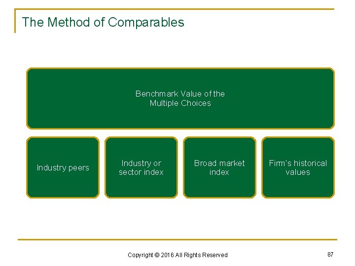
The Method of Comparables Benchmark Value of the Multiple Choices Industry peers Industry or sector index Broad market index Copyright © 2016 All Rights Reserved Firm’s historical values 87

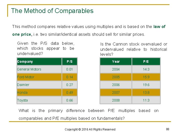
The Method of Comparables This method compares relative values using multiples and is based on the law of one price, i. e. two similar/identical assets should sell for similar prices. Given the P/S data below, which stocks appear to be undervalued? Is the Cannon stock overvalued or undervalued relative to historical levels? Company P/S Year P/E General Motors 0. 01 2004 14. 3 Ford Motor 0. 14 2005 15. 9 Daimler 0. 27 2006 19. 6 Honda 0. 49 2007 13. 8 Toyota 0. 66 2008 11. 3 What is the primary difference between P/E multiples based on comparables and P/E multiples based on fundamentals? Copyright © 2016 All Rights Reserved 88

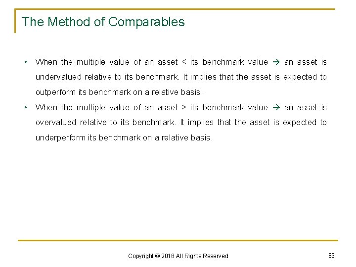
The Method of Comparables • When the multiple value of an asset < its benchmark value an asset is undervalued relative to its benchmark. It implies that the asset is expected to outperform its benchmark on a relative basis. • When the multiple value of an asset > its benchmark value an asset is overvalued relative to its benchmark. It implies that the asset is expected to underperform its benchmark on a relative basis. Copyright © 2016 All Rights Reserved 89

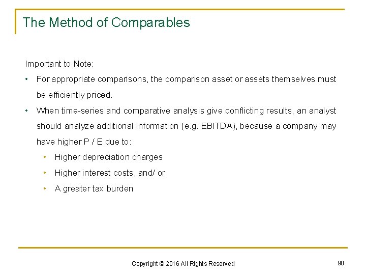
The Method of Comparables Important to Note: • For appropriate comparisons, the comparison asset or assets themselves must be efficiently priced. • When time-series and comparative analysis give conflicting results, an analyst should analyze additional information (e. g. EBITDA), because a company may have higher P / E due to: • Higher depreciation charges • Higher interest costs, and/ or • A greater tax burden Copyright © 2016 All Rights Reserved 90

The Method of Comparables: Advantages • Price multiples facilitate analysts and investors to make relative comparisons both on cross-sectional and time-series basis. • Price multiples are easy to calculate. • Price multiplies are readily available from financial websites and newspapers. Copyright © 2016 All Rights Reserved 91

The Method of Comparables: Limitations • This method only gives relative investment recommendations. However, the stock may be undervalued relative to its benchmark but overvalued when compared to its estimate of intrinsic value as determined by its fundamentals. • Due to differences in reporting rules and accounting methods among different markets, price multiples are not easily comparable. • Multiples for cyclical companies may be highly sensitive to current economic conditions. Copyright © 2016 All Rights Reserved 92

Drawbacks of using P/E ratio • EPS can be negative. The P/E ratio is not meaningful when a denominator is negative. • Earnings are affected by changes in business cycles and often have volatile, transient components which make the analysis difficult. • Earnings are extremely sensitive to fixed operating and financing costs (operating & financial leverage). • Earnings are subject to accounting manipulations to improve company’s performance. • As a result, during periods of economic slowdown or extraordinary growth, it is preferred to use P/S multiple because sales cannot be negative and during extreme situations, change in sales will be less than the change in earnings in % terms. Copyright © 2016 All Rights Reserved 93

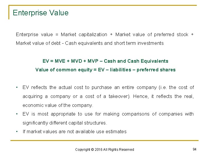
Enterprise Value Enterprise value = Market capitalization + Market value of preferred stock + Market value of debt - Cash equivalents and short term investments EV = MVE + MVD + MVP – Cash and Cash Equivalents Value of common equity = EV – liabilities – preferred shares • EV reflects the actual cost to purchase an entire company (i. e. the cost of acquiring a company or a cost of a takeover). Hence, it reflects the real, economic value of the company. • EV is most appropriate to use for making comparisons of companies with significantly different capital structures. • If market values are not available use estimates Copyright © 2016 All Rights Reserved 94

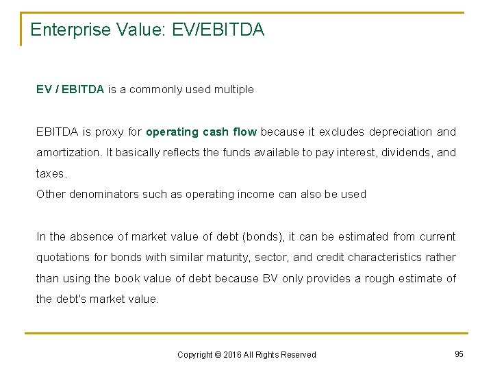
Enterprise Value: EV/EBITDA EV / EBITDA is a commonly used multiple EBITDA is proxy for operating cash flow because it excludes depreciation and amortization. It basically reflects the funds available to pay interest, dividends, and taxes. Other denominators such as operating income can also be used In the absence of market value of debt (bonds), it can be estimated from current quotations for bonds with similar maturity, sector, and credit characteristics rather than using the book value of debt because BV only provides a rough estimate of the debt's market value. Copyright © 2016 All Rights Reserved 95

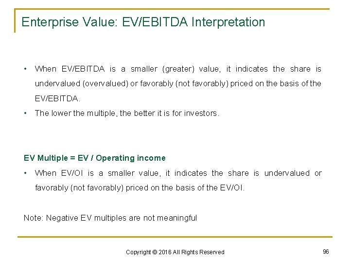
Enterprise Value: EV/EBITDA Interpretation • When EV/EBITDA is a smaller (greater) value, it indicates the share is undervalued (overvalued) or favorably (not favorably) priced on the basis of the EV/EBITDA. • The lower the multiple, the better it is for investors. EV Multiple = EV / Operating income • When EV/OI is a smaller value, it indicates the share is undervalued or favorably (not favorably) priced on the basis of the EV/OI. Note: Negative EV multiples are not meaningful Copyright © 2016 All Rights Reserved 96

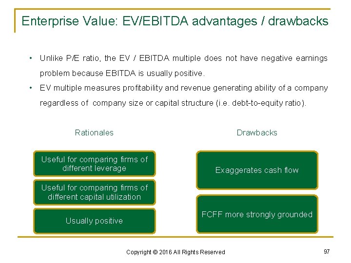
Enterprise Value: EV/EBITDA advantages / drawbacks • Unlike P/E ratio, the EV / EBITDA multiple does not have negative earnings problem because EBITDA is usually positive. • EV multiple measures profitability and revenue generating ability of a company regardless of company size or capital structure (i. e. debt-to-equity ratio). Rationales Drawbacks Useful for comparing firms of different leverage Exaggerates cash flow Useful for comparing firms of different capital utilization Usually positive FCFF more strongly grounded Copyright © 2016 All Rights Reserved 97

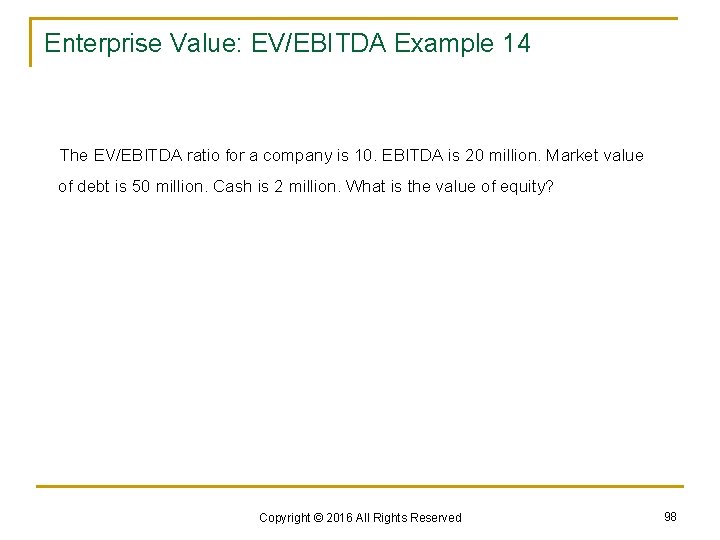
Enterprise Value: EV/EBITDA Example 14 The EV/EBITDA ratio for a company is 10. EBITDA is 20 million. Market value of debt is 50 million. Cash is 2 million. What is the value of equity? Copyright © 2016 All Rights Reserved 98

EV/EBITDA Example 15 Nectar – Fructal Case (Excel) Copyright © 2016 All Rights Reserved 99

6. ASSET-BASED VALUATION Copyright © 2016 All Rights Reserved 100

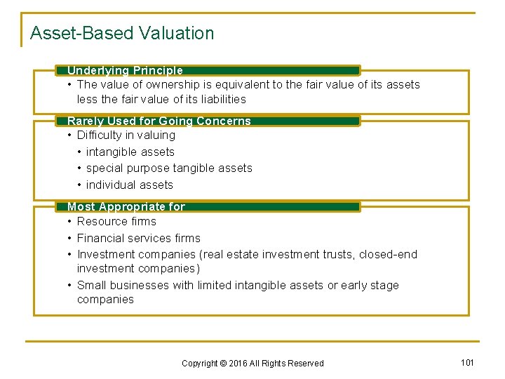
Asset-Based Valuation Underlying Principle • The value of ownership is equivalent to the fair value of its assets less the fair value of its liabilities Rarely Used for Going Concerns • Difficulty in valuing • intangible assets • special purpose tangible assets • individual assets Most Appropriate for • Resource firms • Financial services firms • Investment companies (real estate investment trusts, closed-end investment companies) • Small businesses with limited intangible assets or early stage companies Copyright © 2016 All Rights Reserved 101

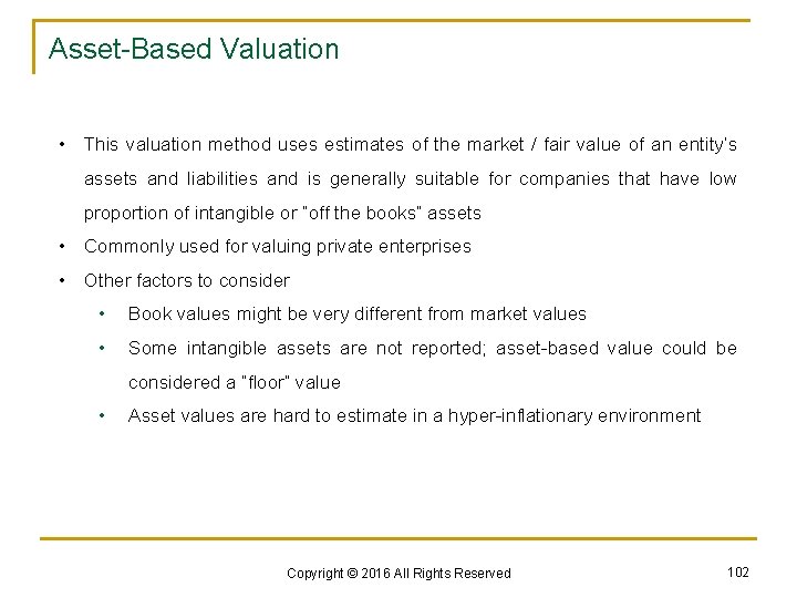
Asset-Based Valuation • This valuation method uses estimates of the market / fair value of an entity’s assets and liabilities and is generally suitable for companies that have low proportion of intangible or “off the books” assets • Commonly used for valuing private enterprises • Other factors to consider • Book values might be very different from market values • Some intangible assets are not reported; asset-based value could be considered a “floor” value • Asset values are hard to estimate in a hyper-inflationary environment Copyright © 2016 All Rights Reserved 102

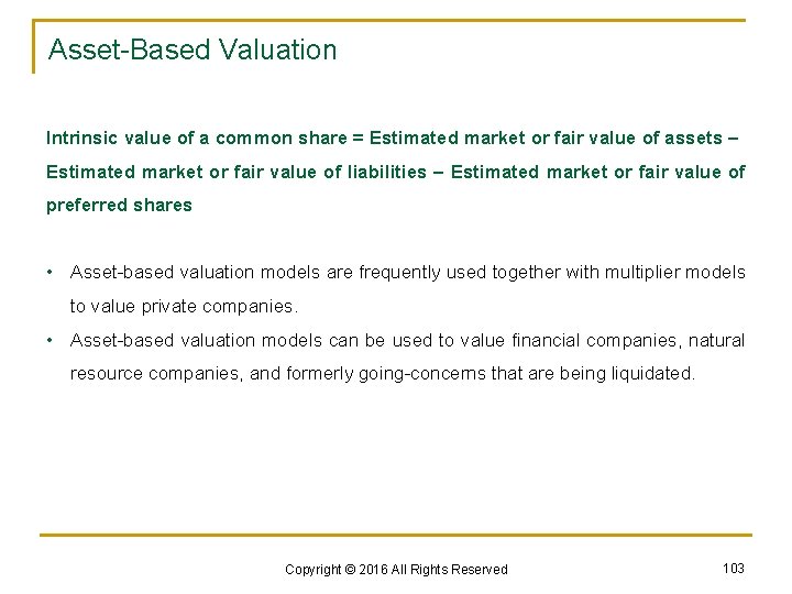
Asset-Based Valuation Intrinsic value of a common share = Estimated market or fair value of assets – Estimated market or fair value of liabilities – Estimated market or fair value of preferred shares • Asset-based valuation models are frequently used together with multiplier models to value private companies. • Asset-based valuation models can be used to value financial companies, natural resource companies, and formerly going-concerns that are being liquidated. Copyright © 2016 All Rights Reserved 103

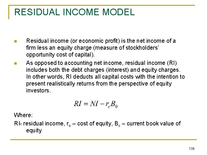
RESIDUAL INCOME MODEL n n Residual income (or economic profit) is the net income of a firm less an equity charge (measure of stockholders’ opportunity cost of capital). As opposed to accounting net income, residual income (RI) includes both the debt charges (interest) and equity charges. In other words, RI deducts all capital costs with the intention to present realistically returns from the perspective of equity investors. Where: RI- residual income, re – cost of equity, Bo – current book value of equity 104

7. SUMMARY AND CONCLUSION Copyright © 2016 All Rights Reserved 105

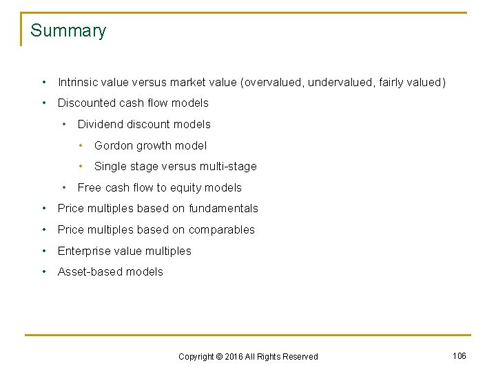
Summary • Intrinsic value versus market value (overvalued, undervalued, fairly valued) • Discounted cash flow models • Dividend discount models • Gordon growth model • Single stage versus multi-stage • Free cash flow to equity models • Price multiples based on fundamentals • Price multiples based on comparables • Enterprise value multiples • Asset-based models Copyright © 2016 All Rights Reserved 106

Conclusion • Review key objectives • Read summary • Memorize formulas • Examples and practice problems from the curriculum (EOC) is highly recommended • Review material and practice questions from other relevant sources Copyright © 2016 All Rights Reserved 107

Thank you for your kind cooperation! Copyright © 2016 All Rights Reserved 108