EQUILIBRIUM OF A FIRM Firm is said to

EQUILIBRIUM OF A FIRM • Firm is said to be in equilibrium when it has no tendency either to increase or to contract its output. • Firm’s equilibrium level of output will lie where its money profits are maximum. • Now profits are the difference between total revenue and total cost. • So in order to be in equilibrium, the firm will attempt to maximise the difference between total revenue and total cost.

• An old method of explaining the equilibrium of the firm is to draw the total revenue and total cost curves of the firm and locate the maximum profit point. • But, with the appearance of Marginalist Revolution, equilibrium of the firm is explained with the aid of marginal revenue and marginal cost curves.

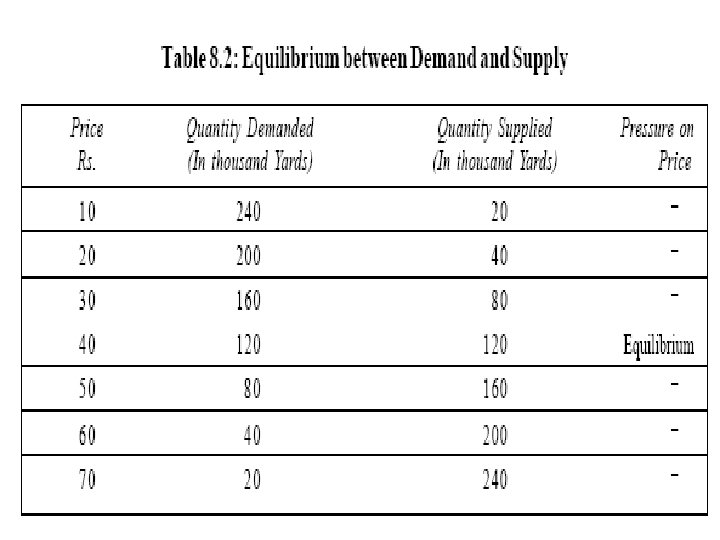
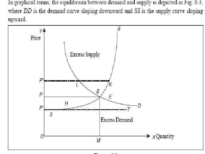
• Demand supply are in equilibrium at point E where two curves intersect each other. • It means that only at price of the quantity demanded is equal to quantity supplied. •

• OM is the equilibrium quantity which is exchanged at price OP. If the price is greater than the equilibrium price say OP”, the quantity demanded by the buyers is P”L, while the quantity offered to supply is P”K. Thus LK is the excess supply which the buyers will not take at the price OP”. • Thus there will be a tendency for the price to fall to the level of equilibrium price OP.

• At price OP’, which is less than the equilibrium price, the buyers demand P’T, the sellers are prepared to supply only P’H. HT represents excess demand. • The unsatisfied buyers will compete with each other to obtain the limited supply of cloth and in this effort they will bid up the price. • Thus, we see that price is determined by the equilibrium between demand supply.

Nature of Revenue curves • Under perfect competition, the market price is determined by the market forces namely the demand for and the supply of the products. • Hence there is uniform price in the market and all the units of the output are sold at the same price. As a result the average revenue is perfectly elastic.

• The average revenue curve is horizontally parallel to X-axis. Since the Average Revenue is constant, Marginal Revenue is also constant and coincides with Average Revenue. • AR curve of a firm represents the demand curve for the product produced by that firm.

Short run equilibrium price and output determination under perfect competition 1. Since a firm in the perfectly competitive market is a price-taker, it has to adjust its level of output to maximise its profit. The aim of any producer is to maximise his profit. • 2. The short run is a period in which the number and plant size of the firms are fixed. In this period, the firm can produce more only by increasing the variable inputs • 3. As the entry of new firms or exit of the existing firms are not possible in the short-run, the firm in the perfectly competitive market can either earn supernormal profit or incur loss in the short period

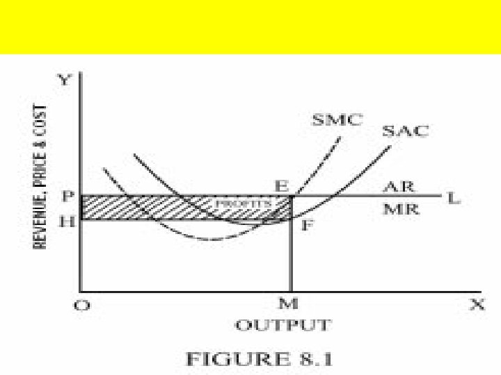
• In figure 8. 1, output is measured along the x-axis and price, revenue and cost along the y-axis. OP is the prevailing price in the market. PL is the demand curve or average and the marginal revenue curve. SAC and SMC are the short run average and marginal cost curves. • The firm is in equilibrium at point ‘E’ where MR = MC and MC curve cuts MR curve from below at the point of equilibrium. Therefore the firm will be producing OM level of output.

• At the OM level of output ME is the AR and MF is the average cost. The profit per unit of output is EF (the difference between ME and MF). • The total profits earned by the firm will be equal to EF (profit per unit) multiplied by OM or HF (total output). Thus the total profits will be equal to the area HFEP is the supernormal profits earned by the firm.

Revenue of a Competitive Firm Total revenue for a firm is the selling price times the quantity sold. TR = (P X Q)

Revenue of a Competitive Firm Marginal revenue is the change in total revenue from an additional unit sold. MR = TR/ Q

Revenue of a Competitive Firm For competitive firms, marginal revenue equals the price of the good.

Total, Average, and Marginal Revenue for a Competitive Firm

Profit Maximization for the Competitive Firm u. The goal of a competitive firm is to maximize profit. u. This means that the firm will want to produce the quantity that maximizes the difference between total revenue and total cost.

Profit Maximization: A Numerical Example

Profit Maximization for the Competitive Firm. . . Costs and Revenue The firm maximizes profit by producing the quantity at which marginal cost equals marginal revenue. MC MC 2 ATC P=MR 1 P = AR = MR AVC MC 1 0 Q 1 QMAX Q 2 Quantity

Profit Maximization for the Competitive Firm • Profit maximization occurs at the quantity where marginal revenue equals marginal cost.

Profit Maximization for the Competitive Firm When MR > MC increase Q When MR < MC decrease Q When MR = MC Profit is maximized. The firm produces up to the point where MR=MC

Monopoly • While a competitive firm is a price taker, a monopoly firm is a price maker.

Monopoly • A firm is considered a monopoly if. . . ¼it is the sole seller of its product. ¼its product does not have close substitutes.

Characteristics of Monopoly • 1. Single Seller: There is only one seller; he can control either price or supply of his product. But he cannot control demand for the product, as there are many buyers. • 2. No close Substitutes: There are no close substitutes for the product. The buyers have no alternatives or choice. Either they have to buy the product or go without it.

3. Price: • The monopolist has control over the supply so as to increase the price. Sometimes he may adopt price discrimination. He may fix different prices for different sets of consumers. • A monopolist can either fix the price or quantity of output; but he cannot do both, at the same time.

4. No Entry: • There is no freedom to other producers to enter the market as the monopolist is enjoying monopoly power. There are strong barriers for new firms to enter. • There are legal, technological, economic and natural obstacles, which may block the entry of new producers.

5. Firm and Industry: • Under monopoly, there is no difference between a firm and an industry. As there is only one firm, that single firm constitutes the whole industry

Why Monopolies Arise Barriers to entry have three sources: • Ownership of a key resource. – This tends to be rare. SCV is an example • The government gives a single firm the exclusive right to produce some good. – Patents, Copyrights and Government Licensing. • Costs of production make a single producer more efficient than a large number of producers. – Natural Monopolies

Economies of Scale as a Cause of Monopoly. . . Cost Average total cost 0 Quantity of Output

Monopoly versus Competition Monopoly Competitive Firm u Is the sole producer u. Is one of many u Has a downward-sloping producers demand curve u. Has a horizontal u Is a price maker demand curve u Reduces price to u. Is a price taker increase sales u. Sells as much or as little at same price

Demand Curves for Competitive and Monopoly Firms. . . Price (a) A Competitive Firm’s Demand Curve (b) A Monopolist’s Demand Curve Price Demand 0 Quantity of Output

A Monopoly’s Revenue • Total Revenue P x Q = TR • Average Revenue TR/Q = AR = P • Marginal Revenue DTR/DQ = MR

A Monopoly’s Marginal Revenue • A monopolist’s marginal revenue is always less than the price of its good. u. The demand curve is downward sloping. u. When a monopoly drops the price to sell one more unit, the revenue received from previously sold units also decreases.

A Monopoly’s Marginal Revenue • A monopolist’s marginal revenue is always less than the price of its good. u. The demand curve is downward sloping. u. When a monopoly drops the price to sell one more unit, the revenue received from previously sold units also decreases.

A Monopoly’s Total, Average, and Marginal Revenue Quantity (Q) 0 1 2 3 4 5 6 7 8 Price (P) $11. 00 $10. 00 $9. 00 $8. 00 $7. 00 $6. 00 $5. 00 $4. 00 $3. 00 Total Revenue (TR=Px. Q) $0. 00 $18. 00 $24. 00 $28. 00 $30. 00 $28. 00 $24. 00 Average Revenue (AR=TR/Q) $10. 00 $9. 00 $8. 00 $7. 00 $6. 00 $5. 00 $4. 00 $3. 00 Marginal Revenue (MR= DTR / )DQ $10. 00 $8. 00 $6. 00 $4. 00 $2. 00 $0. 00 -$2. 00 -$4. 00

A Monopoly’s Marginal Revenue • When a monopoly increases the amount it sells, it has two effects on total revenue (P x Q). u. The output effect—more output is sold, so Q is higher. u. The price effect—price falls, so P is lower.

A Monopoly’s Marginal Revenue • When a monopoly increases the amount it sells, it has two effects on total revenue (P x Q). u. The output effect—more output is sold, so Q is higher. u. The price effect—price falls, so P is lower.

Demand Marginal Revenue Curves for a Monopoly. . . Price $11 10 9 8 7 6 5 4 3 2 1 0 -1 -2 -3 -4 Demand (average revenue) Marginal revenue 1 2 3 4 5 6 7 8 Quantity of Water

Harcourt, Inc. items and derived items copyright © 2001 by Harcourt, Inc. Profit-Maximization for a Monopoly. . . 2. . and then the demand curve shows the price consistent with this quantity. Costs and Revenue B Monopoly price 1. The intersection of the marginal-revenue curve and the marginal-cost curve determines the profit-maximizing quantity. . . Average total cost A Demand Marginal cost Marginal revenue 0 QMAX Quantity

Comparing Monopoly and Competition • For a competitive firm, price equals marginal cost. P = MR = MC • For a monopoly firm, price exceeds marginal cost. P > MR = MC

A Monopoly’s Profit • • Profit equals total revenue minus total costs. Profit = TR - TC Profit = (TR/Q - TC/Q) x Q Profit = (P - ATC) x Q

. The Monopolist’s Profit. . . Costs and Revenue Marginal cost E B y ol op on fit M pro Monopoly price Average total cost D Average total cost C Demand Marginal revenue 0 QMAX Quantity

The Monopolist’s Profit • The monopolist will receive economic profits as long as price is greater than average total cost.

Marginal-Cost Pricing for a Natural Monopoly. . . Price Average total cost Loss Regulated price Average total cost Marginal cost Demand 0 Quantity

Price Discrimination • Price discrimination is the practice of selling the same good at different prices to different customers, even though the costs for producing for the two customers are the same. In order to do this, the firm must have market power.

Price Discrimination • • Two important effects of price discrimination: u. It can increase the monopolist’s profits. u. It can reduce deadweight loss. But in order to price discriminate, the firm must u. Be able to separate the customers on the basis of willingness to pay. u. Prevent the customers from reselling the product.

The Early Bird Gets a Lower Price • Early Bird Specials— Restaurants charge special, lower prices for early diners. • Matinees—Theaters charge less for earlier shows. • Air Fares—Airlines charge less for flyers willing to fly “off peak, ” i. e. early morning and late night.

Is Price Discrimination Always Undesirable? • No, although sometimes justice appears to demand different prices in different markets. • In some cases, price discrimination may be necessary for a firm to survive. • In some cases, where there are significant economies of scale, price discrimination may actually lead to lower prices.

THE ANATOMY OF FACTOR MARKETS – The four factors of production that produce goods and services are: • Labor • Capital • Land • Entrepreneurship

THE ANATOMY OF FACTOR MARKETS – Factor price – The price of a factor of production. • The wage rate is the price of labor. • The interest rate is the price of capital. • Rent is the price of land. – Factor market – A market for labor, capital, or land.

THE ANATOMY OF FACTOR MARKETS • Labor Markets –Labor market –A collection of people and firms who are trading labor services. –Job –A contract between a firm and a household to provide labor services.

THE ANATOMY OF FACTOR MARKETS • Financial Markets –Capital –The tools, instruments, machines, and other constructions that have been produced in the past and that businesses use to produce goods and services. –Financial capital –The funds that firms use to buy and operate physical capital.

THE ANATOMY OF FACTOR MARKETS – Financial Market –A collection of people and firms who are lending and borrowing to finance the purchase of physical capital. –The two main types of financial market are • Stock market • Bond market

THE ANATOMY OF FACTOR MARKETS –Stock Market –A stock market is a market in which the shares in the stocks of companies are traded. –Examples: MSE CSE. SEBI

THE ANATOMY OF FACTOR MARKETS –Bond Market –A bond market is a market in which bonds issued by firms or governments are traded. –Bond –A promise to pay specified sums of money on specified dates.

THE ANATOMY OF FACTOR MARKETS • Land Markets –Land consists of all the gifts of nature. –A market in which raw materials are traded are called a commodity market. • Competitive Factor Markets –Most factor markets have many buyers and sellers and are competitive markets.

DEMAND FOR A FACTOR OF PRODUCTION – Derived demand – The demand for a factor of production, which is derived from the demand for the goods and services it is used to produce. – Value of marginal product – The value to a firm of hiring one more unit of a factor of production, which equals price of a unit of output multiplied by the marginal product of the factor of production.

DEMAND FOR A FACTOR OF PRODUCTION • Value of Marginal Product –Table on the next slide walks you through the calculation of the value of marginal product.

DEMAND FOR A FACTOR OF PRODUCTION The first two columns of the table are the firm’s total product schedule. To calculate marginal product, find the change in total product as the quantity of labor increases by 1 worker.

DEMAND FOR A FACTOR OF PRODUCTION To calculate the value of marginal product, multiply the marginal product numbers by the price of a car wash, which in this example is Rs. 3.

DEMAND FOR A FACTOR OF PRODUCTION

DEMAND FOR A FACTOR OF PRODUCTION Figure shows the value of the marginal product at Max’s Wash ’n’ Wax. The blue bars show the value of the marginal product of the labor that Max hires based on the numbers in the table.

DEMAND FOR A FACTOR OF PRODUCTION The orange line is the firm’s value of the marginal product of labor curve.

DEMAND FOR A FACTOR OF PRODUCTION • A Firm’s Demand for Labor – A firm hires labor up to the point at which the value of marginal product equals the wage rate. – If the value of marginal product of labor exceeds the wage rate, a firm can increase its profit by employing one more worker. – If the wage rate exceeds the value of marginal product of labor, a firm can increase its profit by employing one fewer worker.

DEMAND FOR A FACTOR OF PRODUCTION –A Firm’s Demand for Labor Curve –A firm’s demand for labor curve is also its value of marginal product curve. –If the wage rate falls, a firm hires more workers.

DEMAND FOR A FACTOR OF PRODUCTION Figure shows the demand for labor at Max’s Wash’n’ Wax. At a wage rate of Rs 10. 50 an hour, Max makes a profit on the first 2 workers but would incur a loss on the third worker.

18. 2 DEMAND FOR A FACTOR OF PRODUCTION Figure 18. 2 shows the demand for labor at Max’s Wash’n’ Wax. At a wage rate of $10. 50 an hour, Max makes a profit on the first 2 workers but would incur a loss on the third worker. So Max’s quantity of labor demanded is 2 workers. Max’s demand for labor curve is the same as the value of marginal product curve.

DEMAND FOR A FACTOR OF PRODUCTION The demand for labor curve slopes downward because the value of the marginal product of labor diminishes as the quantity of labor employed increases.

DEMAND FOR A FACTOR OF PRODUCTION –Changes in the Demand for Labor –The demand for labor depends on: • The price of the firm’s output • The prices of other factors of production • Technology

DEMAND FOR A FACTOR OF PRODUCTION –The Price of the Firm’s Output –The higher the price of a firm’s output, the greater is its demand for labor. –The Prices of Other Factors of Production –If the price of using capital decreases relative to the wage rate, a firm substitutes capital for labor and increases the quantity of capital it uses. –Usually, the demand for labor will decrease when the price of using capital falls.

DEMAND IN FACTOR MARKET –Technology –New technologies decrease the demand for some types of labor and increase the demand for other types.

WAGES AND EMPLOYMENT • The Supply of Labor – People supply labor to earn an income. Many factors influence the quantity of labor that a person plans to provide, but the wage rate is a key factor. – Figure 18. 3 on the next slide shows an individual’s labor supply curve.

WAGES AND EMPLOYMENT The table shows Larry’s labor supply schedule, which is plotted in the figure as Larry’s labor supply curve.

18. 3 WAGES AND EMPLOYMENT 1. At a wage rate of $10. 50 an hour, Larry … 2. …supplies 30 hours of labor a week.

18. 3 WAGES AND EMPLOYMENT 3. As the wage rate rises, Larry’s quantity of labor supplied … 4. …increases, 5. …reaches a maximum, … 6. …then decreases.

18. 3 WAGES AND EMPLOYMENT Larry’s labor supply curve eventually bends backward.

18. 3 WAGES AND EMPLOYMENT –Market Supply Curve –A market supply curve shows the quantity of labor supplied by all households in a particular job. –It is found by adding together the quantities of labor supplied by all households at each wage rate. –Figure 18. 4 on the next slide shows the supply of car wash workers.

18. 3 WAGES AND EMPLOYMENT This supply curve shows how the quantity of car wash workers supplied changes when the wage rate changes, other things remaining the same.

18. 3 WAGES AND EMPLOYMENT In a market for a specific type of labor, the quantity supplied increases as the wage rate increases, other things remaining the same.

18. 3 WAGES AND EMPLOYMENT • Influences on the Supply of Labor – Three key factors influence the supply of labor: • Adult population • Preferences • Time in school and training

18. 3 WAGES AND EMPLOYMENT –Adult Population –An increase in the adult population increases the supply of labor. –Preferences –There has been a large increase in the supply of female labor since 1960. –The percentage of men with jobs has shrunk slightly.

18. 3 WAGES AND EMPLOYMENT –Time in School and Training –The more people who remain in school for fulltime education and training, the smaller is the supply of low-skilled labor.

18. 3 WAGES AND EMPLOYMENT • Labor Market Equilibrium – Labor market equilibrium determines the wage rate and employment. – Figure 18. 5 on the next slide illustrates equilibrium in the market for car wash workers.

18. 3 WAGES AND EMPLOYMENT 1. The equilibrium wage rate is $10. 50 an hour. 2. The equilibrium quantity of labor is 300 workers.

18. 3 WAGES AND EMPLOYMENT If the wage rate exceeds $10. 50 an hour, the quantity demanded is less than the quantity supplied and the wage rate falls. If the wage rate is below $10. 50 an hour, the quantity demanded exceeds the quantity supplied and the wage rate rises.

18. 4 FINANCIAL MARKETS • The Demand for Financial Capital – A firm’s demand for financial capital stems from its demand for physical capital to produce goods and services. – The quantity of physical capital that a firm plans to use depends on the price of financial capital—the interest rate. – Two factors that change the demand for captial are: • Population growth • Technological change

18. 4 FINANCIAL MARKETS • The Supply of Financial Capital – The quantity of financial capital supplied results from people’s saving decisions. – The higher the interest rate, the greater is the quantity of saving supplied. – The main influences on the supply of saving are: • Population • Average income • Expected future income

18. 4 FINANCIAL MARKETS • Financial Market Equilibrium and the Interest Rate – Financial market equilibrium occurs when the interest rate has adjusted to make the quantity of capital demanded equal the quantity of capital supplied. – Figure 18. 6 on the next slide illustrates financial market equilibrium.

18. 4 FINANCIAL MARKETS The demand for financial capital is KD, and the supply of financial capital is KS. 1. The equilibrium interest rate is 6 percent a year. 2. The equilibrium quantity of financial capital is $200 billion.

18. 5 LAND NATURAL RESOURCE MARKETS – All natural resources are called land, and they fall into two categories: • Renewable • Nonrenewable – Renewable natural resources – Natural resources that can be used repeatedly. – Nonrenewable natural resources – Natural resources that can be used only once and that cannot be replaced once they have been used.

18. 5 LAND NATURAL RESOURCE MARKETS • The Market for Land (Renewable Natural Resources) – The lower the rent, the greater is the quantity of land demanded. – The supply of a particular block of land is perfectly inelastic. – Figure 18. 7 illustrates this market for land.

18. 5 LAND NATURAL RESOURCE MARKETS The demand curve for a 10 -acre block of land is D, and the supply curve is S. Equilibrium occurs at a rent of $1, 000 an acre per day.

18. 5 LAND NATURAL RESOURCE MARKETS • Economic Rent and Opportunity Cost – Economic rent – The income received by any factor of production over and above the amount required to induce a given quantity of the factor to be supplied. – The income that is required to induce the supply of a given quantity of a factor of production is its opportunity cost—the value of the factor of production in its next best use.

18. 5 LAND NATURAL RESOURCE MARKETS Figure 18. 8 shows how the income of a factor of production divides between economic rent and opportunity cost. 1. Part of the income is opportunity cost (the red area). 2. Part is economic rent (the green area).

18. 5 LAND NATURAL RESOURCE MARKETS • The Supply of a Nonrenewable Resource – Over time, the quantity of a nonrenewable resource decreases as it is used up. – But the known quantity of a natural resource increases because advances in technology enable ever less accessible sources of the resource to be discovered. – Using a natural resource decreases its supply, which causes price to rise. – New discoveries increase supply, which cause prices to fall.

Factor Markets in YOUR Life Would you like to be a millionaire? If so, it is in factor markets that you are going to make it happen. You might come up with a $1 million idea—borrow to finance capital expenditure and hire labor. But the surest way is by saving. If, starting at age 25, you save $66 a week and earn interest at 8 percent a year, how will it take to accumulate $1 million? 40 years! You’ll be a millionaire at age 65. By making the capital market work for you, you can grow a few dollars a week into $1 million.

Market Structure

Market Structure • Market structure – identifies how a market is made up in terms of: The number of firms in the industry The nature of the product produced The degree of monopoly power each firm has The degree to which the firm can influence price Profit levels Firms’ behaviour – pricing strategies, non-price competition, output levels – The extent of barriers to entry – The impact on efficiency – – –

Market Structure Perfect Competition Pure Monopoly More competitive (fewer imperfections)

Market Structure Perfect Competition Pure Monopoly Less competitive (greater degree of imperfection)

Market Structure Pure Monopoly Perfect Competition Monopolistic Competition Oligopoly Duopoly Monopoly The further right on the scale, the greater the degree of monopoly power exercised by the firm.

Market Structure • Importance: • Degree of competition affects the consumer – will it benefit the consumer or not? • Impacts on the performance and behaviour of the company/companies involved

Market Structure • Models – a word of warning! – Market structure deals with a number of economic ‘models’ – These models are a representation of reality to help us to understand what may be happening in real life – There are extremes to the model that are unlikely to occur in reality – They still have value as they enable us to draw comparisons and contrasts with what is observed in reality – Models help therefore in analysing and evaluating – they offer a benchmark

Market Structure • Characteristics of each model: – Number and size of firms that make up the industry – Control over price or output – Freedom of entry and exit from the industry – Nature of the product – degree of homogeneity (similarity) of the products in the industry (extent to which products can be regarded as substitutes for each other) – Diagrammatic representation – the shape of the demand curve, etc.

Market Structure Characteristics: Look at these everyday products – what type of market structure are the producers of these products operating in? Mercedes CLK Coupe Remember to think about the nature of the product, entry and exit, behaviour of the firms, number and size of the firms in the industry. Canon SLR Camera Bananas You might even have to ask what the industry is? ? Electric Guitar – Jazz Body Vodka

Perfect Competition • One extreme of the market structure spectrum • Characteristics: – Large number of firms – Products are homogenous (identical) – consumer has no reason to express a preference for any firm – Freedom of entry and exit into and out of the industry – Firms are price takers – have no control over the price they charge for their product – Each producer supplies a very small proportion of total industry output – Consumers and producers have perfect knowledge about the market

Perfect Competition Diagrammatic representation Cost/Revenue MC AC Given The average The the MC industry assumption is the cost price curve of ofisprofit isfirm the At. The this output the maximisation, standard producing determined ‘U’ –additional the shaped by firm the produces curve. demand making normal atis MC an (marginal) cuts output and the supply where AC units of curve MC of theoutput. = industry at. MR its It profit. This is a long (Q 1). lowest falls as This at point a first whole. output because (due level The to firm the is of athe law is a of fraction mathematical diminishing very of the small total relationship returns) supplier industry then within rises run equilibrium supply. between asthe output industry marginal rises. andhas average no position. values. control over price. They will sell each extra unit for the same price. Price therefore = MR and AR P = MR = AR Q 1 Output/Sales

Perfect Competition Diagrammatic representation Cost/Revenue MC MC 1 AC AC 1 abnormal profit. If new firms enter the industry, will Nowlower The Because assume ACmodel aand firmsupply MC makes assumes would increase, price willisfall and the some that imply perfect form knowledge, the of modification firm the now firmto firm will leftgains making its product earning gains thebe abnormal advantage or profit some fornormal only form a profit once again. of costtime (AR>AC) short advantage represented before others (sayby acopy new the production grey the idea area. or method). are attracted What to the would happen? industry by the existence of Average and Marginal costs could be expected to be lower but price, in the short run, remains the same. P = MR = AR Abnormal profit P 1 = MR 1 = AR 1 Q 2 Output/Sales

Monopolistic or Imperfect Competition • Where the conditions of perfect competition do not hold, ‘imperfect competition’ will exist • Varying degrees of imperfection give rise to varying market structures • Monopolistic competition is one of these – not to be confused with monopoly!

Monopolistic or Imperfect Competition • Characteristics: – Large number of firms in the industry – May have some element of control over price due to the fact that they are able to differentiate their product in some way from their rivals – products are therefore close, but not perfect, substitutes – Entry and exit from the industry is relatively easy – few barriers to entry and exit – Consumer and producer knowledge imperfect

Monopolistic or Imperfect Competition Implications for the diagram: MC Cost/Revenue AC £ 1. 00 Abnormal Profit £ 0. 60 MR Q 1 D (AR) Output / Sales We Marginal assume Cost that and the firmand This If. Since The the is firm demand a the short produces additional run curve equilibrium Q 1 facing produces Average where Cost will MR be the position sells the firm revenue each forwill received aunit firm befor downward in£ 1. 00 from a = MC on (profit same maximising shape. However, output). monopolistic average sloping each unit with and sold market represents thefalls, cost structure. the (onthe At because this output the level, products AR>AC average) AR MR earned curve forlies from each under sales. unit the being and are the differentiated firm makes in 60 p, AR curve. the firm will make 40 p x abnormal way, profit the(the firmgrey will Q 1 some in abnormal profit. shaded only be area). able to sell extra output by lowering price.

Monopolistic or Imperfect Competition Implications for the diagram: Cost/Revenue MC AC MR 1 MR Q 1 AR 1 D (AR) Output / Sales Because there is relative freedom of entry and exit into the market, new firms will enter encouraged by the existence of abnormal profits. New entrants will increase supply causing price to fall. As price falls, the AR and MR curves shift inwards as revenue from each sale is now less.

Monopolistic or Imperfect Competition Implications for the diagram: Cost/Revenue MC AC AR = AC MR 1 Q 2 MR Q 1 AR 1 D (AR) Output / Sales Notice that the existence of more substitutes makes the new AR (D) curve more price elastic. The firm reduces output to a point where MC = MR (Q 2). At this output AR = AC and the firm will make normal profit.

Monopolistic or Imperfect Competition Implications for the diagram: Cost/Revenue MC AC AR = AC MR 1 Q 2 AR 1 Output / Sales This is the long run equilibrium position of a firm in monopolistic competition.

Monopolistic or Imperfect Competition • Some important points about monopolistic competition: – May reflect a wide range of markets – Not just one point on a scale – reflects many degrees of ‘imperfection’ – Examples?

• • • Monopolistic or Imperfect Competition Restaurants Plumbers/electricians/local builders Solicitors Private schools Plant hire firms Insurance brokers Health clubs Hairdressers Funeral directors Estate agents Damp proofing control firms

Monopolistic or Imperfect Competition • In each case there are many firms in the industry • Each can try to differentiate its product in some way • Entry and exit to the industry is relatively free • Consumers and producers do not have perfect knowledge of the market – the market may indeed be relatively localised. Can you imagine trying to search out the details, prices, reliability, quality of service, etc for every plumber in the UK in the event of an emergency? ?

Oligopoly • Competition between the few – May be a large number of firms in the industry but the industry is dominated by a small number of very large producers • Concentration Ratio – the proportion of total market sales (share) held by the top 3, 4, 5, etc firms: – A 4 firm concentration ratio of 75% means the top 4 firms account for 75% of all the sales in the industry

Oligopoly • Example: • Music sales – The music industry has a 5 -firm concentration ratio of 75%. Independents make up 25% of the market but there could be many thousands of firms that make up this ‘independents’ group. An oligopolistic market structure therefore may have many firms in the industry but it is dominated by a few large sellers. Market Share of the Music Industry 2002. Source IFPI: http: //www. ifpi. org/site-content/press/20030909. html

Oligopoly • Features of an oligopolistic market structure: – Price may be relatively stable across the industry – kinked demand curve? – Potential for collusion – Behaviour of firms affected by what they believe their rivals might do – interdependence of firms – Goods could be homogenous or highly differentiated – Branding and brand loyalty may be a potent source of competitive advantage – Non-price competition may be prevalent – Game theory can be used to explain some behaviour – AC curve may be saucer shaped – minimum efficient scale could occur over large range of output – High barriers to entry

Oligopoly Price The kinked demand curve - an explanation for price stability? The Assume If The thefirm principle therefore, seeks firm ofto is the lower charging effectively kinked its price demand a faces price to of £ 5‘kinked gain a and acurve competitive producing demand rests on an curve’ advantage, the output principle forcing of its 100. itrivals to will follow maintain that: asuit. stable Anyorgains rigid pricing it makes will If it chose to raise price above £ 5, its quickly be. Oligopolistic structure. lost and the firms % change may in rivals not followitssuit andits the firm a. would If a firm raises price, demand will overcome this beby smaller engaging thaninthe non% effectively an follow elasticsuit demand rivalsfaces will not reduction price competition. in price – total revenue would curve for its product (consumers would again b. fall If a as firmthe lowers firm now its price, facesits a buy from the cheaper rivals). The % relatively rivals inelastic will all demand do the same curve. change in demand would be greater than the % change in price and TR would fall. £ 5 Total Revenue B Total Revenue A Total Revenue B Kinked D Curve D = elastic D = Inelastic 100 Quantity

Duopoly • Market structure where the industry is dominated by two large producers – Collusion may be a possible feature – Price leadership by the larger of the two firms may exist – the smaller firm follows the price lead of the larger one – Highly interdependent – High barriers to entry – Cournot Model – French economist – analysed duopoly – suggested long run equilibrium would see equal market share and normal profit made – In reality, local duopolies may exist

Monopoly • Pure monopoly – where only one producer exists in the industry • In reality, rarely exists – always some form of substitute available! • Monopoly exists, therefore, where one firm dominates the market • Firms may be investigated for examples of monopoly power when market share exceeds 25% • Use term ‘monopoly power’ with care!

Monopoly • Monopoly power – refers to cases where firms influence the market in some way through their behaviour – determined by the degree of concentration in the industry Influencing prices Influencing output Erecting barriers to entry Pricing strategies to prevent or stifle competition May not pursue profit maximisation – encourages unwanted entrants to the market – Sometimes seen as a case of market failure – – –

Monopoly • Origins of monopoly: – Through growth of the firm – Through amalgamation, merger or takeover – Through acquiring patent or license – Through legal means – Royal charter, nationalisation, wholly owned plc

Monopoly • Summary of characteristics of firms exercising monopoly power: – Price – could be deemed too high, may be set to destroy competition (destroyer or predatory pricing), price discrimination possible. – Efficiency – could be inefficient due to lack of competition (X- inefficiency) or… • could be higher due to availability of high profits

Monopoly • Innovation - could be high because of the promise of high profits, Possibly encourages high investment in research and development (R&D) • Collusion – possible to maintain monopoly power of key firms in industry • High levels of branding, advertising and non-price competition

Monopoly • Problems with models – a reminder: – Often difficult to distinguish between a monopoly and an oligopoly – both may exhibit behaviour that reflects monopoly power – Monopolies and oligopolies do not necessarily aim for traditional assumption of profit maximisation – Degree of contestability of the market may influence behaviour – Monopolies not always ‘bad’ – may be desirable in some cases but may need strong regulation – Monopolies do not have to be big – could exist locally

Monopoly Costs / Revenue MC £ 7. 00 AC Monopoly Profit This(D) AR Given isthe both curve barriers the forshort a to monopolist entry, run and likely the long monopolist run to be equilibrium relatively will be position price able to inelastic. exploit for a monopoly abnormal Output assumed profits in the to be atrun long profit as maximising entry to the output (note caution market is restricted. here – not all monopolists may aim for profit maximisation!) £ 3. 00 MR Q 1 AR Output / Sales

Monopoly Welfare implications of monopolies Costs / Revenue MC £ 7 AC Loss of consumer surplus £ 3 AR MR Q 2 A look back at the for The higher price monopoly in price a competitive price anddiagram lower would be perfect competition will reveal output market £ 7 permeans unit would with that beoutput £ 3 consumer with levels output that in equilibrium, price will be surplus levels at lower at is Q 2. Q 1. reduced, indicated by equal to the MC of production. the grey shaded area. On the face of it, consumers We can look therefore at a face higher prices and less comparison of the differences choice in monopoly conditions between price and output in a compared to more competitive situation compared environments. to a monopoly. Q 1 Output / Sales

Monopoly Welfare implications of monopolies Costs / Revenue MC £ 7 AC Gain in producer surplus The monopolist will benefit be affected from additional by a loss producer of producer surplus equal showntobythe thegrey triangle but……. . shaded rectangle. £ 3 AR MR Q 2 Q 1 Output / Sales

Monopoly Welfare implications of monopolies Costs / Revenue MC £ 7 AC The value of the grey shaded triangle represents the total welfare loss to society – sometimes referred to as the ‘deadweight welfare loss’. £ 3 AR MR Q 2 Q 1 Output / Sales

Contestable Markets • Theory developed by William J. Baumol, John Panzar and Robert Willig (1982) • Helped to fill important gaps in market structure theory • Perfectly contestable market – the pure form – not common in reality but a benchmark to explain firms’ behaviours

Contestable Markets • Key characteristics: – Firms’ behaviour influenced by the threat of new entrants to the industry – No barriers to entry or exit – No sunk costs – Firms may deliberately limit profits made to discourage new entrants – entry limit pricing – Firms may attempt to erect artificial barriers to entry – e. g…

Contestable Markets • Over capacity – provides the opportunity to flood the market and drive down price in the event of a threat of entry • Aggressive marketing and branding strategies to ‘tighten’ up the market • Potential for predatory or destroyer pricing • Find ways of reducing costs and increasing efficiency to gain competitive advantage

Contestable Markets • ‘Hit and Run’ tactics – enter the industry, take the profit and get out quickly (possible because of the freedom of entry and exit) • Cream-skimming – identifying parts of the market that are high in value added and exploiting those markets

Contestable Markets • Examples of markets exhibiting contestability characteristics: – Financial services – Airlines – especially flights on domestic routes – Computer industry – ISPs, software, web development – Energy supplies – The postal service?

Market Structures • Final reminders: • • • Models can be used as a comparison – they are not necessarily meant to BE reality! When looking at real world examples, focus on the behaviour of the firm in relation to what the model predicts would happen – that gives the basis for analysis and evaluation of the real world situation. Regulation – or the threat of regulation may well affect the way a firm behaves. Remember that these models are based on certain assumptions – in the real world some of these assumptions may not be valid, this allows us to draw comparisons and contrasts. The way that governments deal with firms may be based on a general assumption that more competition is better than less!