Equality Function Computation How to make simple things

Equality Function Computation (How to make simple things complicated) Nitin Vaidya University of Illinois at Urbana-Champaign Joint work with Guanfeng Liang Research supported in part by National Science Foundation and Army Research Office

Background 2

Equality Function A B K-valued input Determine whether the two inputs are identical 3

g Communication cost of an algorithm: # bits of communication required in the worst case (over all possible inputs) 4

g Communication cost of an algorithm: # bits of communication required in the worst case (over all possible inputs) g Communication complexity of a problem: Minimum communication cost over all algorithms to solve the problem [Andrew Yao, STOC 1979]

Equality Function A B K-valued input 6

Upper Bound A log K B Proof by construction 7

Lower Bound A log K B Proof by fooling set argument 8

Generalization to n parties 9

The MEQ(n, K) Problem g g n nodes each given xi from {1, …, K}, to check if all xi are equal Each node i computes EQi “Everyone detects” (MEQ-ED) 10

The MEQ(n, K) Problem g g n nodes each given xi from {1, …, K}, to check if all xi are equal Each node i computes EQi “Anyone detects” (MEQ-AD) 11

n-Node Equality Problem B A Network C 12

Number-in-Hand Model K-valued input A Broadcast Channel B C Node i initially knows Xi 13

n-Party Equality : Complexity g Broadcast channel + Number-in-hand model log K bits 14

Number-on-Forehead Model A Broadcast Channel B C Node i initially knows everything except Xi 15

n-Party Equality : Complexity g Broadcast channel + Number-on-forehead model 2 bits when n > 2 16

Point-to-Point Networks Private channels & number-in-hand B A n=3 C 17

Upper Bound Emulate broadcast channel using p 2 p links (n-1) * complexity with broadcast channel 18

Upper Bound = 2 log K K-valued input A log K bits B log K bits C 19

Lower Bound = log K K-valued input B A cut log K by 2 -node lower bound C identical value at B and C 20

1. 5 log K Complexity B A Neither bound tight in general 2 log K C 21

1. 5 log K Not Tight B A K=2 C Requires at least 2 bits 22

2 log K Not Tight B A C Proof by construction for K = 6 2 log K = log 36

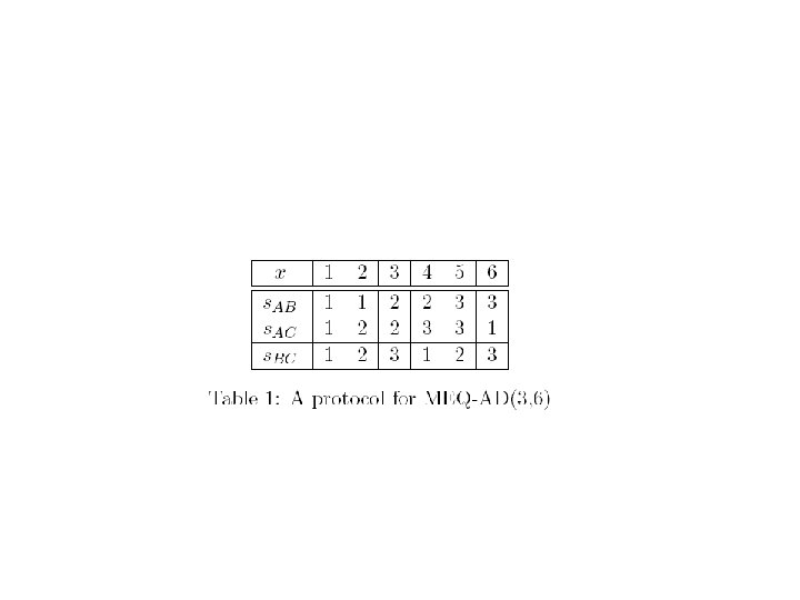
K=6 x y A B C z 1 2 3 4 5 6 AB 1 1 2 2 3 3 AC 1 2 2 3 3 1 BC 1 2 3

Example 3 4 A B C 3 1 2 3 4 5 6 AB 1 1 2 2 3 3 AC 1 2 2 3 3 1 BC 1 2 3

Example 3 4 2 A B C 3 1 2 3 4 5 6 AB 1 1 2 2 3 3 AC 1 2 2 3 3 1 BC 1 2 3

Example 3 4 2 A B 2 C 3 1 2 3 4 5 6 AB 1 1 2 2 3 3 AC 1 2 2 3 3 1 BC 1 2 3

Example 3 4 2 A B 1 2 C 3 1 2 3 4 5 6 AB 1 1 2 2 3 3 AC 1 2 2 3 3 1 BC 1 2 3

Example 3 4 2 A B AB(4) = 2 AC(2) = 3 BC(3) = 1 1 2 C 3 1 2 3 4 5 6 AB 1 1 2 2 3 3 AC 1 2 2 3 3 1 BC 1 2 3

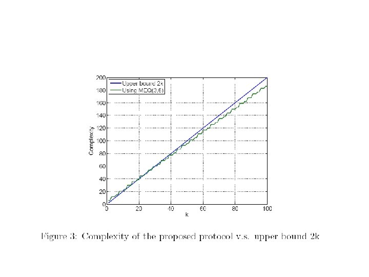
Communication Cost 3 log 3 = log 27 < log 36 = 2 log K Can be generalized to large K and n to yield communication cost approximately 0. 92 (n-1) log K 30

Communication Cost 3 log 3 = log 27 < log 36 = 2 log K Can be generalized to large K and n to yield communication cost approximately 0. 92 (n-1) log K Cost of informing outcome to each other negligible for large K 31

1 2 3 4 5 6 AB 1 1 2 2 3 3 AC 1 2 2 3 3 1 BC 1 2 3

Reduce Search Space “Static” Protocols g Node transmitting in round R its output function in round R pre-determined & i. Output … function of initial input, and history 33

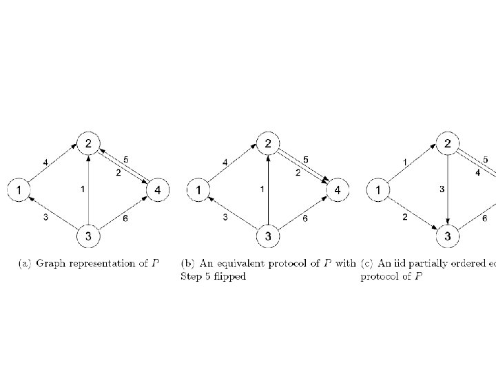
Static Protocol: Directed Graph Representation y B 1, f 1 4, f 4 5, f 5 A x 6, f 6 2, f 2 3, f 3 C Round number R , function f used in round R z 34

Static Protocol: Directed Graph Representation y B 1, f 1 4, f 4 5, f 5 A x 6, f 6 2, f 2 3, f 3 C Round number R , function f used in round R z 35

Equivalent Protocol: Directed Acyclic Graph y B 1, f 1 4, f 4 5, f 5 A x 6, f 6 2, f 2 3, f 3 C Round number R , function f used in round R z 36

Equivalent Protocol g g Acyclic graph Output depends only on initial input B FAB A FAC FBC C 37

Mapping to a Bipartite Graph g Each such protocol can be mapped to a bipartite graph representation B FAB A FAC FBC C 38

Example 1 2 3 4 5 6 AB 1 1 2 2 3 3 AC 1 2 2 3 3 1 BC 1 2 3 1, 2 3, 4 5, 6 AB 39

Example 1 2 3 4 5 6 AB 1 1 2 2 3 3 AC 1 2 2 3 3 1 BC 1 2 3 1, 2 6, 1 3, 4 2, 3 5, 6 4, 5 AB AC 40

Example 1 2 3 4 5 6 AB 1 1 2 2 3 3 AC 1 2 2 3 3 1 BC 1 2 3 1 1, 2 6, 1 2 3 3, 4 2, 3 6 5, 6 AB 4 5 4, 5 AC 41

Example 1 2 3 4 5 6 AB 1 1 2 2 3 3 AC 1 2 2 3 3 1 BC 1 2 3 1 1, 2 2 3 3, 4 2, 3 6 5, 6 BC 3 2 1 6, 1 AB 4 5 BC 4, 5 AC 42

BC assigns colors to edges 1 2 3 4 5 6 AB 1 1 2 2 3 3 AC 1 2 2 3 3 1 BC 1 2 3 1 1, 2 2 3 3, 4 2, 3 6 5, 6 BC 3 2 1 6, 1 AB 4 5 BC 4, 5 AC 43

U : # nodes on left V : # colors W : # nodes on right U 3 V 3 W 3 1 1, 2 6, 1 2 3 3, 4 2, 3 6 5, 6 BC 3 2 1 AB 4 5 BC 4, 5 AC 44

Equality Bipartite Graph A colored bipartite graph corresponds to a fixed protocol for 3 -node equality with cost log UVW if and only if (a) (b) (c) (d) (e) distance-2 colored Number of edges = K Ux. V ≥ K Ux. W ≥ K Vx. W ≥ K (strong edge coloring) 45

Fixed Protocol Design g Find a suitable bipartite graph g Our protocol 6 -cycle 46

Lower Bounds g The mapping can be used to prove lower bounds for small K For K = 6 g Least cost over all fixed protocols is log 27 47

Detour … an open conjecture A bipartite graph with g g D 1 = maximum degree on left D 2 = maximum degree on right can be distance-2 colored with D 1 * D 2 colors 48

Why is equality interesting ? 49

Lower Bound on Consensus g Mapping between Byzantine broadcast and multiple instances of equality 50

g g 1 – g 3 are good peers F 1 – F 3 are virtual bad sources acting with different inputs gi, j are virtual good peer of node j to node i

Byzantine Broadcast: n nodes, f faults g Broadcast algorithm solves Equality (MEQAD)problem for each subset of (n-f) nodes g n-choose-(n-f) such subsets Each link belongs to (n-2)-choose-(n-f-2) such subsets Complexity of broadcast lower bounded by g EQ * n-choose-(n-f) / (n-2)-choose-(n-f-2) 52

Open Problems 53

Open Problems g Characterizations of communication complexity for point-to-point networks i. Alternatives to Yao model seem more appropriate g Equality for larger networks g Lower bounds on i. Equality i. Byzantine consensus i. Byzantine broadcast … 54

Thanks ! 55

Thanks ! 56

57

58

59

60

61

The MEQ(n, M) Problem g g n nodes each given xi from {1, …, M}, to check if all xi are equal Each node i computes EQi “Anyone detects” (MEQ-AD) 62

Graph Representation an Algorithm g 2 g 1, f 1 g 5, g 4, g 2, f 5 f 2 f 4 g 6, f 6 g 1 g 3, f 3 g. Transform to a partially ordered DAG 63

Graph Representation an Algorithm g 2 g. F 1, 2 g 1 g. F 2, 3 g. F 1, 3 g. Fi, j depends on xi only 64

Definition of Complexity g Complexity of an algorithm g Complexity of MEQ(n, M) 65

Upper Bound by Construction g Send x 1, …, xn-1 to node n g Set EQ 1 = … = EQn-1 = 0 g Compute EQn = EQ(x 1, …, xn) g 66

Cut-Set Lower Bound g Fooling Set argument - Every node must send + receive ≥ log 2 M g 67

Neither bound is tight MEQ(3, 6) g 2 g. F 1, 2 g 1 g. F 2, 3 g. F 1, 3 g 3 68

Proof by Strong Edge Coloring MEQ(3, M) algorithm = bipartite graph with M edges + distance-2 edge coloring scheme F 1, 2 2 F 1, 3 6, 1 2 F 2, 3 1 1 1, 2 3 3, 4 2, 3 6 3 5, 6 F 1, 2 4 5 F 2, 3 4, 5 69 F 1, 3

Summary g Introduce the MEQ problem g Existing techniques give loose bounds g New technique to reduce space g Connection among distributed source coding, distributed algorithm, and graph coloring 70

Future Work g MEQ(3, M) is open i. Optimize over Fi, j = find an optimal bipartite graph + strong coloring g Even given |Fi, j| is open g Looking for new techniques 71