Episode 6 Parallel operations Parallel conjunction and disjunction

6. 1 Parallel conjunction and disjunction A B and A B are simultaneous (parallel)

6. 2 Which game is the easiest for the machine to win? Comparing, by

6. 3 Free versus strict games We say that a game is strict iff,

6. 4 Chess: a really easy game The copycat (mimicking) strategy wins the game!

6. 5 Resource-counsciusness Classical logic is resource-blind: it sees no difference between, say, A

6. 6 Differences with linear logic #1 #2 #3 #4 #5 #6 #7 #8

6. 7 Parallel quantifiers Parallel universal quantifier : x. A(x) = A(0) A(1) A(2)

6. 8 Parallel conjunction and disjunction defined Below and later we use the notation

6. 9 Parallel quantifiers defined Definition 6. 9. a Let A(x)=(Vr, A) be a

6. 10 De. Morgan’s laws for parallel operations Thus, as seen from Definitions 6.

6. 11. a Game trees for parallel combinations Such trees tend to be very

6. 11. b Game trees for parallel combinations Such trees tend to be very

6. 12 Evolution trees Drawing evolution trees may be another helpful visualization method. The

6. 12 Evolution sequences Each legal run induces an evolution sequence --- the sequence

6. 13 Evolution sequences Each legal run induces an evolution sequence --- the sequence

6. 14 Evolution sequences for parallel quantification In a similar way can visualize Position

6. 15 Control questions and exercises 1. You should be able to reproduce the

Slides: 44

Download presentation

Episode 6 Parallel operations • Parallel conjunction and disjunction • Free versus strict games • The law of the excluded middle for parallel disjunction • Resource-consciousness • Differences with linear logic • Parallel quantifiers • De. Morgan’s laws for parallel operations • Evolution trees and evolution sequences

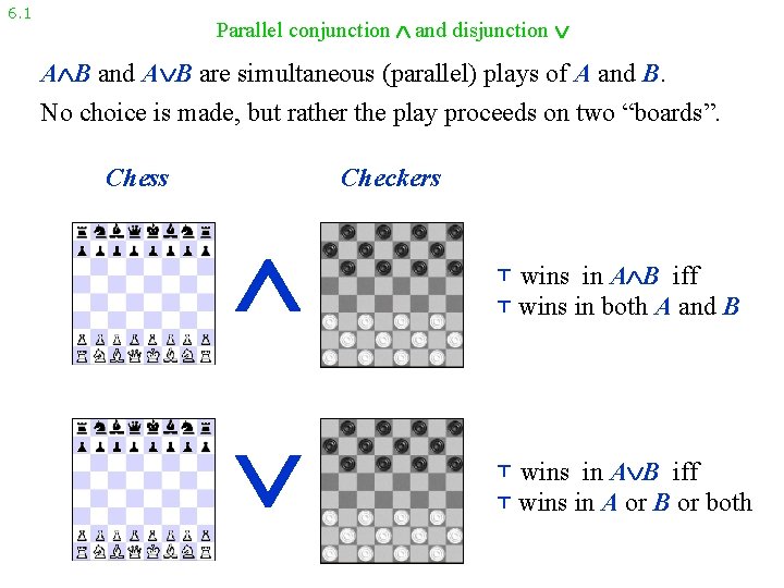
6. 1 Parallel conjunction and disjunction A B and A B are simultaneous (parallel) plays of A and B. No choice is made, but rather the play proceeds on two “boards”. Chess Checkers ⊤ wins in A B iff ⊤ wins in both A and B ⊤ wins in A B iff ⊤ wins in A or B or both

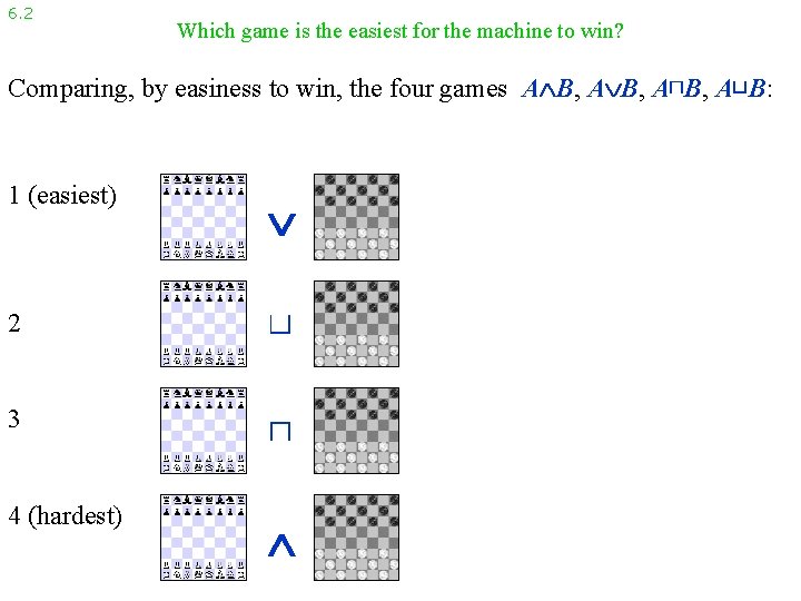
6. 2 Which game is the easiest for the machine to win? Comparing, by easiness to win, the four games A B, A⊓B, A⊔B: 1 (easiest) 2 ⊔ 3 ⊓ 4 (hardest)

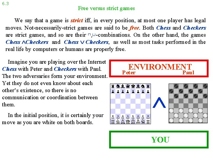
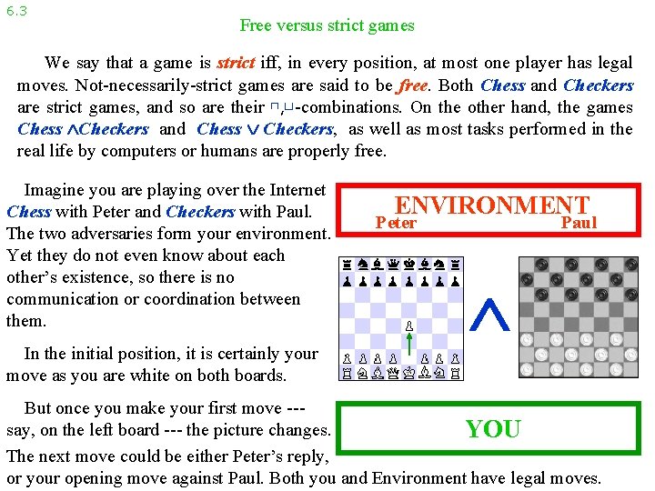
6. 3 Free versus strict games We say that a game is strict iff, in every position, at most one player has legal moves. Not-necessarily-strict games are said to be free. Both Chess and Checkers are strict games, and so are their ⊓, ⊔-combinations. On the other hand, the games Chess Checkers and Chess Checkers, as well as most tasks performed in the real life by computers or humans are properly free. Imagine you are playing over the Internet Chess with Peter and Checkers with Paul. The two adversaries form your environment. Yet they do not even know about each other’s existence, so there is no communication or coordination between them. In the initial position, it is certainly your move as you are white on both boards. ENVIRONMENT Peter Paul YOU

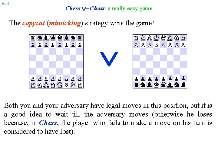
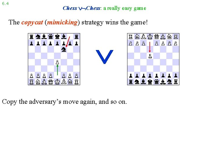
6. 4 Chess: a really easy game The copycat (mimicking) strategy wins the game! Both you and your adversary have legal moves in this position, but it is a good idea to wait till the adversary moves (otherwise he loses because, in Chess, the player who fails to make a move on his turn is considered to have lost).

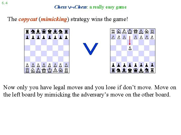
6. 4 Chess: a really easy game The copycat (mimicking) strategy wins the game! Now only you have legal moves and you lose if don’t move. Move on the left board by mimicking the adversary’s move on the other board.

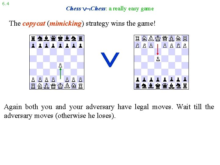
6. 4 Chess: a really easy game The copycat (mimicking) strategy wins the game! Again both you and your adversary have legal moves. Wait till the adversary moves (otherwise he loses).

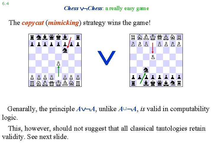
6. 4 Chess: a really easy game The copycat (mimicking) strategy wins the game! Copy the adversary’s move again, and so on.

6. 4 Chess: a really easy game The copycat (mimicking) strategy wins the game! Genarally, the principle A A, unlike A⊔ A, is valid in computability logic. This, however, should not suggest that all classical tautologies retain validity. See next slide.

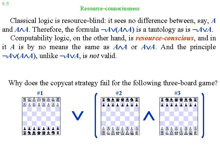
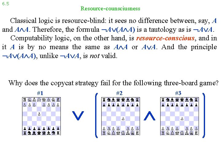
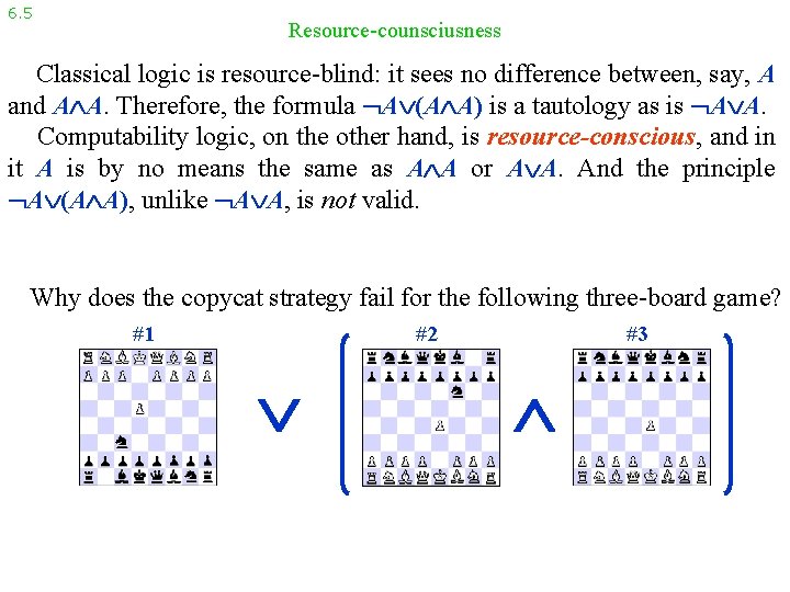
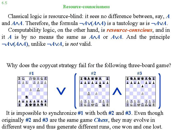
6. 5 Resource-counsciusness Classical logic is resource-blind: it sees no difference between, say, A and A A. Therefore, the formula A (A A) is a tautology as is A A. Computability logic, on the other hand, is resource-conscious, and in it A is by no means the same as A A or A A. And the principle A (A A), unlike A A, is not valid. Why does the copycat strategy fail for the following three-board game? #1 #2 #3 It is impossible to synchronize #1 with both #2 and #3. Even though originally #2 and #3 are the same game Chess, they may evolve in different ways and thus generate different runs, one won and one lost.

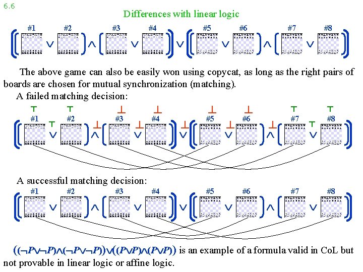
6. 6 Differences with linear logic #1 #2 #3 #4 #5 #6 #7 #8 The above game can also be easily won using copycat, as long as the right pairs of boards are chosen for mutual synchronization (matching). A failed matching decision: ⊤ #1 ⊤ ⊤ #2 ⊥ ⊥ #3 ⊥ ⊥ #4 ⊥ ⊥ #5 ⊥ ⊥ #6 ⊤ ⊥ #7 ⊤ ⊤ #8 A successful matching decision: #1 #2 #3 #4 #5 #6 #7 #8 (( P P)) ((P P)) is an example of a formula valid in Co. L but not provable in linear logic or affine logic.

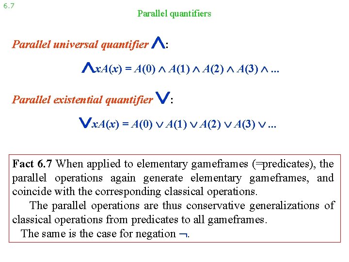
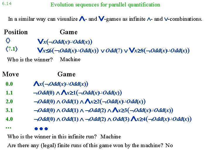
6. 7 Parallel quantifiers Parallel universal quantifier : x. A(x) = A(0) A(1) A(2) A(3) . . . Parallel existential quantifier : x. A(x) = A(0) A(1) A(2) A(3) . . . Fact 6. 7 When applied to elementary gameframes (=predicates), the parallel operations again generate elementary gameframes, and coincide with the corresponding classical operations. The parallel operations are thus conservative generalizations of classical operations from predicates to all gameframes. The same is the case for negation .

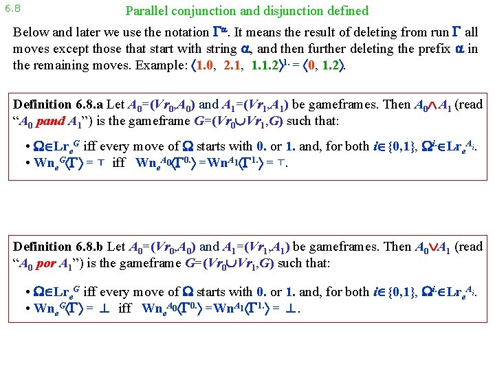
6. 8 Parallel conjunction and disjunction defined Below and later we use the notation . It means the result of deleting from run all moves except those that start with string , and then further deleting the prefix in the remaining moves. Example: 1. 0, 2. 1, 1. 1. 2 1. = 0, 1. 2. Definition 6. 8. a Let A 0=(Vr 0, A 0) and A 1=(Vr 1, A 1) be gameframes. Then A 0 A 1 (read “A 0 pand A 1”) is the gameframe G=(Vr 0 Vr 1, G) such that: • Lre. G iff every move of starts with 0. or 1. and, for both i {0, 1}, i. Lre. Ai. • Wne. G = ⊤ iff Wne. A 0 0. =Wn. A 1 1. = ⊤. Definition 6. 8. b Let A 0=(Vr 0, A 0) and A 1=(Vr 1, A 1) be gameframes. Then A 0 A 1 (read “A 0 por A 1”) is the gameframe G=(Vr 0 Vr 1, G) such that: • Lre. G iff every move of starts with 0. or 1. and, for both i {0, 1}, i. Lre. Ai. • Wne. G = ⊥ iff Wne. A 0 0. =Wn. A 1 1. = ⊥.

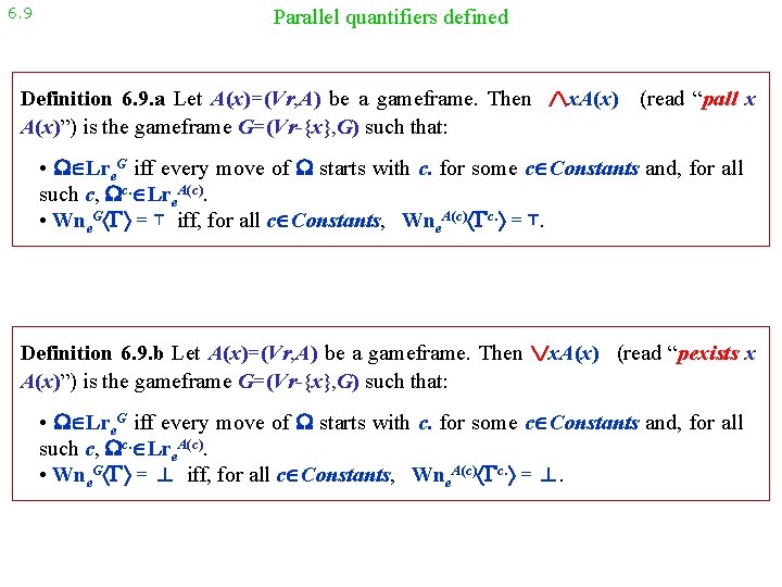
6. 9 Parallel quantifiers defined Definition 6. 9. a Let A(x)=(Vr, A) be a gameframe. Then A(x)”) is the gameframe G=(Vr-{x}, G) such that: x. A(x) (read “pall x • Lre. G iff every move of starts with c. for some c Constants and, for all such c, c. Lre. A(c). • Wne. G = ⊤ iff, for all c Constants, Wne. A(c) c. = ⊤. Definition 6. 9. b Let A(x)=(Vr, A) be a gameframe. Then A(x)”) is the gameframe G=(Vr-{x}, G) such that: x. A(x) (read “pexists x • Lre. G iff every move of starts with c. for some c Constants and, for all such c, c. Lre. A(c). • Wne. G = ⊥ iff, for all c Constants, Wne. A(c) c. = ⊥.

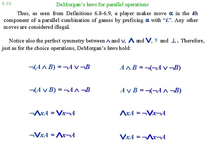
6. 10 De. Morgan’s laws for parallel operations Thus, as seen from Definitions 6. 8 -6. 9, a player makes move in the ith component of a parallel combination of games by prefixing with “i. ”. Any other moves are considered illegal. Notice also the perfect symmetry between and , and just as for the choice operations, De. Morgan’s laws hold: , ⊤ and ⊥. Therefore, (A B) = A B = ( A B) x. A = x A x. A = x A

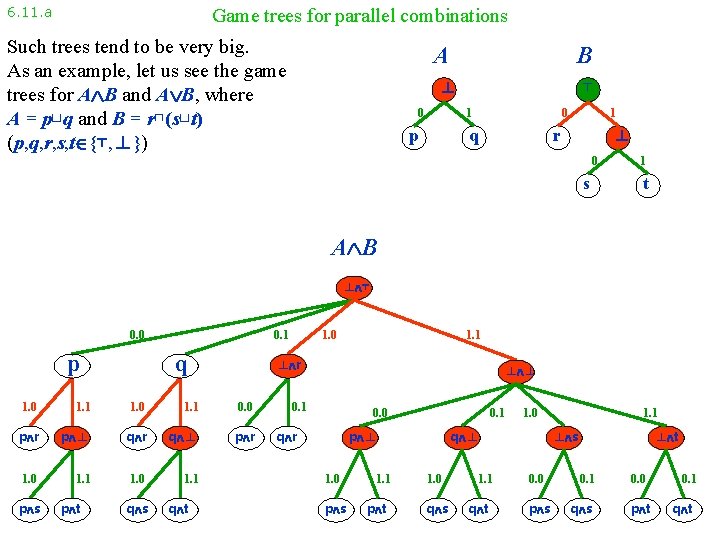
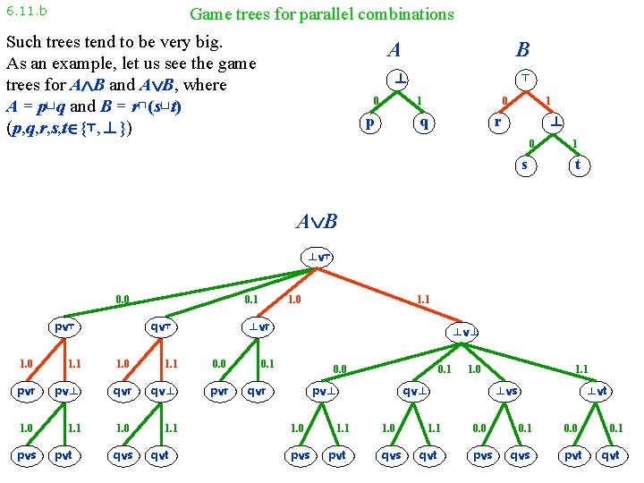
6. 11. a Game trees for parallel combinations Such trees tend to be very big. As an example, let us see the game trees for A B and A B, where A = p⊔q and B = r⊓(s⊔t) (p, q, r, s, t {⊤, ⊥}) A B ⊥ 0 ⊤ 0 1 p q 1 ⊥ r 0 s 1 t A B ⊥ ⊤ 0. 0 p ⊤ 0. 1 q ⊤ 1. 1 1. 0 1. 1 0. 0 p r p ⊥ q r q ⊥ p r 1. 0 1. 1 p t q s q t 1. 1 ⊥ r 1. 0 p s 1. 0 ⊥ ⊥ 0. 1 0. 0 q r 0. 1 p ⊥ 1. 0 p s 1. 1 p t 1. 0 q ⊥ 1. 0 q s 1. 1 q t 1. 1 ⊥ s 0. 0 p s ⊥ t 0. 1 q s 0. 0 p t 0. 1 q t

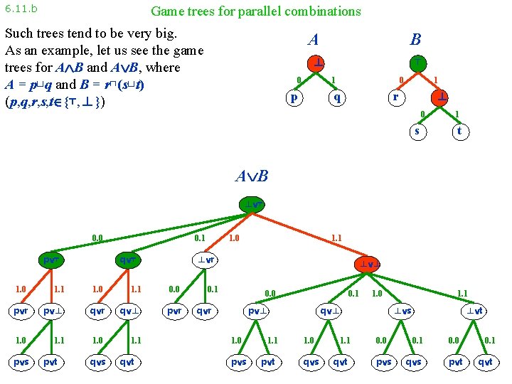
6. 11. a Game trees for parallel combinations Such trees tend to be very big. As an example, let us see the game trees for A B and A B, where A = p⊔q and B = r⊓(s⊔t) (p, q, r, s, t {⊤, ⊥}) A B ⊥ 0 ⊤ 0 1 p q 1 ⊥ r 0 s 1 t A B ⊥ ⊤ 0. 0 p 0. 1 q 1. 1 1. 0 1. 1 0. 0 p r p ⊥ q r q ⊥ p r 1. 0 1. 1 p t q s q t 1. 1 ⊥ r 1. 0 p s 1. 0 ⊥ ⊥ 0. 1 0. 0 q r 0. 1 p ⊥ 1. 0 p s 1. 1 p t 1. 0 q ⊥ 1. 0 q s 1. 1 q t 1. 1 ⊥ s 0. 0 p s ⊥ t 0. 1 q s 0. 0 p t 0. 1 q t

6. 11. b Game trees for parallel combinations Such trees tend to be very big. As an example, let us see the game trees for A B and A B, where A = p⊔q and B = r⊓(s⊔t) (p, q, r, s, t {⊤, ⊥}) A B ⊥ 0 ⊤ 0 1 p q 1 ⊥ r 0 s 1 t A B ⊥ ⊤ 0. 0 p ⊤ 0. 1 q ⊤ 1. 1 1. 0 1. 1 0. 0 p r p ⊥ q r q ⊥ p r 1. 0 1. 1 p t q s q t 1. 1 ⊥ r 1. 0 p s 1. 0 ⊥ ⊥ 0. 1 0. 0 q r 0. 1 p ⊥ 1. 0 p s 1. 1 p t 1. 0 q ⊥ 1. 0 q s 1. 1 q t 1. 1 ⊥ s 0. 0 p s ⊥ t 0. 1 q s 0. 0 p t 0. 1 q t

6. 11. b Game trees for parallel combinations Such trees tend to be very big. As an example, let us see the game trees for A B and A B, where A = p⊔q and B = r⊓(s⊔t) (p, q, r, s, t {⊤, ⊥}) A B ⊥ 0 ⊤ 0 1 p q 1 ⊥ r 0 s 1 t A B ⊥ ⊤ 0. 0 p ⊤ 1. 0 p r 1. 0 p s 1. 1 p t 0. 1 q r 1. 0 q s 1. 1 q 0. 0 p r 1. 1 q t 1. 1 r q ⊤ 1. 0 ⊥ ⊥ 0. 1 p q r 1. 0 p s 0. 0 0. 1 1. 0 q 1. 1 p t 1. 0 q s 1. 1 q t 0. 0 p s 0. 1 q s 0. 0 p t t 0. 1 q t

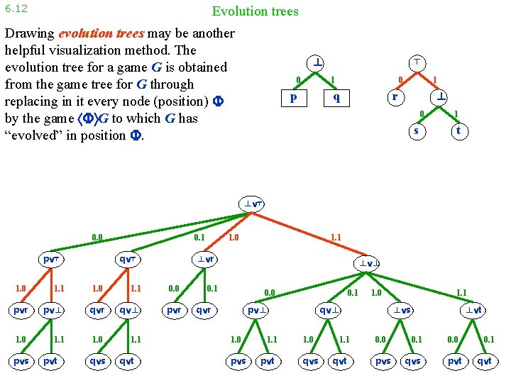
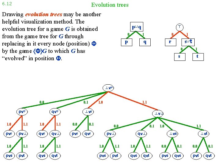
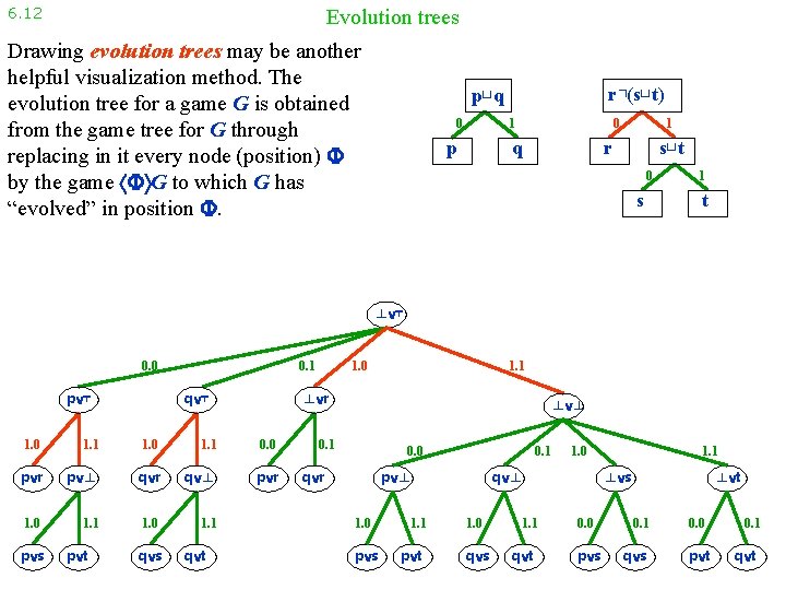
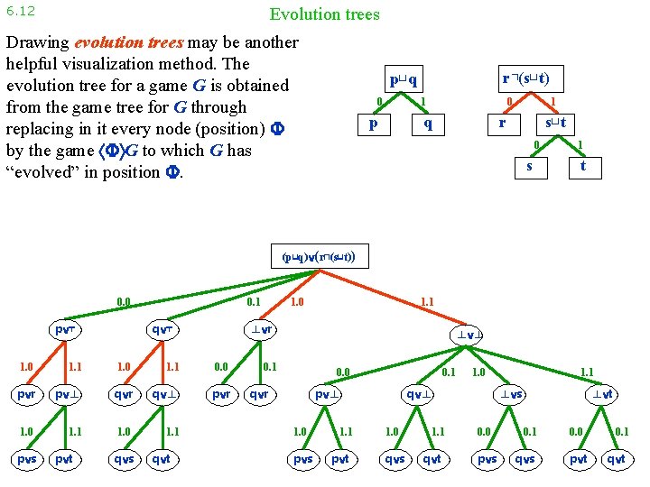
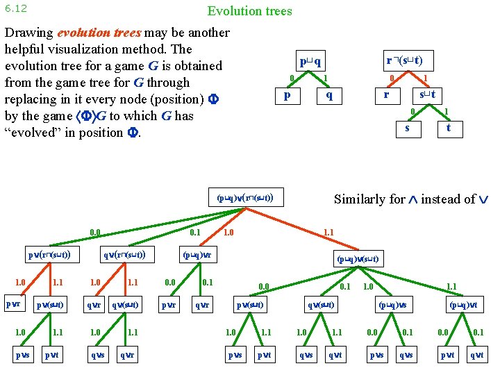
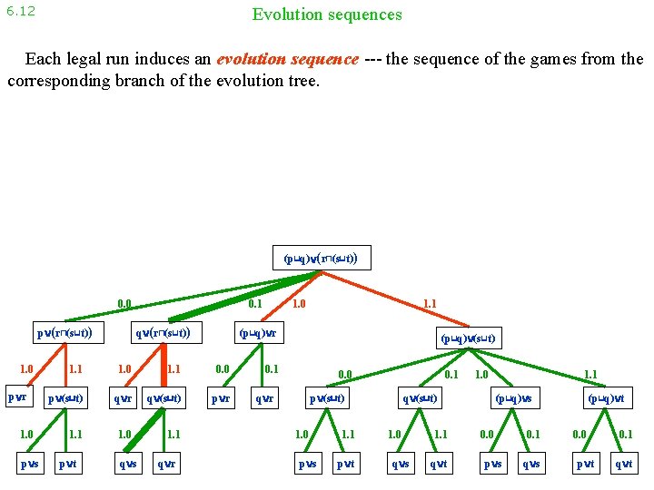
6. 12 Evolution trees Drawing evolution trees may be another helpful visualization method. The evolution tree for a game G is obtained from the game tree for G through replacing in it every node (position) by the game G to which G has “evolved” in position . ⊥ 0 ⊤ 0 1 p q 1 ⊥ r 0 s 1 t ⊥ ⊤ 0. 0 p ⊤ 0. 1 q ⊤ 1. 1 1. 0 1. 1 0. 0 p r p ⊥ q r q ⊥ p r 1. 0 1. 1 p t q s q t 1. 1 ⊥ r 1. 0 p s 1. 0 ⊥ ⊥ 0. 1 0. 0 q r 0. 1 p ⊥ 1. 0 p s 1. 1 p t 1. 0 q ⊥ 1. 0 q s 1. 1 q t 1. 1 ⊥ s 0. 0 p s ⊥ t 0. 1 q s 0. 0 p t 0. 1 q t

6. 12 Evolution trees Drawing evolution trees may be another helpful visualization method. The evolution tree for a game G is obtained from the game tree for G through replacing in it every node (position) by the game G to which G has “evolved” in position . ⊥ 0 ⊤ 0 1 p 1 ⊥ r q 0 s 1 t ⊥ ⊤ 0. 0 p ⊤ 0. 1 q ⊤ 1. 1 1. 0 1. 1 0. 0 p r p ⊥ q r q ⊥ p r 1. 0 1. 1 p t q s q t 1. 1 ⊥ r 1. 0 p s 1. 0 ⊥ ⊥ 0. 1 0. 0 q r 0. 1 p ⊥ 1. 0 p s 1. 1 p t 1. 0 q ⊥ 1. 0 q s 1. 1 q t 1. 1 ⊥ s 0. 0 p s ⊥ t 0. 1 q s 0. 0 p t 0. 1 q t

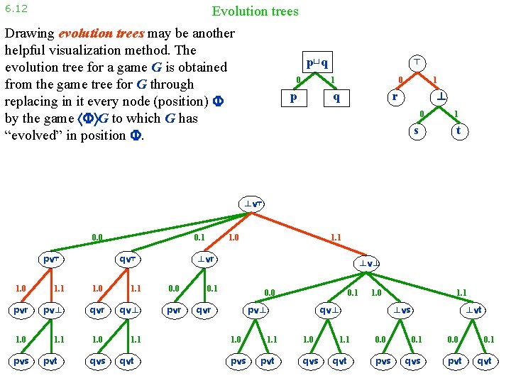
6. 12 Evolution trees Drawing evolution trees may be another helpful visualization method. The evolution tree for a game G is obtained from the game tree for G through replacing in it every node (position) by the game G to which G has “evolved” in position . p⊔q 0 ⊤ 0 1 p 1 ⊥ r q 0 s 1 t ⊥ ⊤ 0. 0 p ⊤ 0. 1 q ⊤ 1. 1 1. 0 1. 1 0. 0 p r p ⊥ q r q ⊥ p r 1. 0 1. 1 p t q s q t 1. 1 ⊥ r 1. 0 p s 1. 0 ⊥ ⊥ 0. 1 0. 0 q r 0. 1 p ⊥ 1. 0 p s 1. 1 p t 1. 0 q ⊥ 1. 0 q s 1. 1 q t 1. 1 ⊥ s 0. 0 p s ⊥ t 0. 1 q s 0. 0 p t 0. 1 q t

6. 12 Evolution trees Drawing evolution trees may be another helpful visualization method. The evolution tree for a game G is obtained from the game tree for G through replacing in it every node (position) by the game G to which G has “evolved” in position . p⊔q 0 ⊤ 0 1 p q 1 s⊔t r 0 s 1 t ⊥ ⊤ 0. 0 p ⊤ 0. 1 q ⊤ 1. 1 1. 0 1. 1 0. 0 p r p ⊥ q r q ⊥ p r 1. 0 1. 1 p t q s q t 1. 1 ⊥ r 1. 0 p s 1. 0 ⊥ ⊥ 0. 1 0. 0 q r 0. 1 p ⊥ 1. 0 p s 1. 1 p t 1. 0 q ⊥ 1. 0 q s 1. 1 q t 1. 1 ⊥ s 0. 0 p s ⊥ t 0. 1 q s 0. 0 p t 0. 1 q t

6. 12 Evolution trees Drawing evolution trees may be another helpful visualization method. The evolution tree for a game G is obtained from the game tree for G through replacing in it every node (position) by the game G to which G has “evolved” in position . r⊓(s⊔t) p⊔q 0 0 1 p q 1 s⊔t r 0 s 1 t ⊥ ⊤ 0. 0 p ⊤ 0. 1 q ⊤ 1. 1 1. 0 1. 1 0. 0 p r p ⊥ q r q ⊥ p r 1. 0 1. 1 p t q s q t 1. 1 ⊥ r 1. 0 p s 1. 0 ⊥ ⊥ 0. 1 0. 0 q r 0. 1 p ⊥ 1. 0 p s 1. 1 p t 1. 0 q ⊥ 1. 0 q s 1. 1 q t 1. 1 ⊥ s 0. 0 p s ⊥ t 0. 1 q s 0. 0 p t 0. 1 q t

6. 12 Evolution trees Drawing evolution trees may be another helpful visualization method. The evolution tree for a game G is obtained from the game tree for G through replacing in it every node (position) by the game G to which G has “evolved” in position . r⊓(s⊔t) p⊔q 0 0 1 p q 1 s⊔t r 0 s 1 t (p⊔q) (r⊓(s⊔t)) 0. 0 p ⊤ 0. 1 q ⊤ 1. 1 1. 0 1. 1 0. 0 p r p ⊥ q r q ⊥ p r 1. 0 1. 1 p t q s q t 1. 1 ⊥ r 1. 0 p s 1. 0 ⊥ ⊥ 0. 1 0. 0 q r 0. 1 p ⊥ 1. 0 p s 1. 1 p t 1. 0 q ⊥ 1. 0 q s 1. 1 q t 1. 1 ⊥ s 0. 0 p s ⊥ t 0. 1 q s 0. 0 p t 0. 1 q t

6. 12 Evolution trees Drawing evolution trees may be another helpful visualization method. The evolution tree for a game G is obtained from the game tree for G through replacing in it every node (position) by the game G to which G has “evolved” in position . r⊓(s⊔t) p⊔q 0 0 1 p q p (r⊓(s⊔t)) 1. 0 p r 1. 0 p s 0. 1 q (r⊓(s⊔t)) 0 s 1. 0 1. 1 0. 0 p (s⊔t) q r q (s⊔t) p r 1. 1 1. 0 1. 1 p t q s q r 1 t Similarly for instead of 1. 0 1. 1 (p⊔q) r 1. 1 s⊔t r (p⊔q) (r⊓(s⊔t)) 0. 0 1 (p⊔q) (s⊔t) 0. 1 0. 0 q r 0. 1 p (s⊔t) 1. 0 p s 1. 1 p t 1. 0 q (s⊔t) 1. 0 q s 1. 1 q t 1. 1 (p⊔q) s 0. 0 p s 0. 1 q s (p⊔q) t 0. 0 p t 0. 1 q t

6. 12 Evolution sequences Each legal run induces an evolution sequence --- the sequence of the games from the corresponding branch of the evolution tree. (p⊔q) (r⊓(s⊔t)) 0. 0 p (r⊓(s⊔t)) 1. 0 p r 1. 0 p s 0. 1 q (r⊓(s⊔t)) 1. 0 1. 1 0. 0 p (s⊔t) q r q (s⊔t) p r 1. 1 1. 0 1. 1 q s q r 1. 1 (p⊔q) r 1. 1 p t 1. 0 (p⊔q) (s⊔t) 0. 1 0. 0 q r 0. 1 p (s⊔t) 1. 0 p s 1. 1 p t 1. 0 q (s⊔t) 1. 0 q s 1. 1 q t 1. 1 (p⊔q) s 0. 0 p s 0. 1 q s (p⊔q) t 0. 0 p t 0. 1 q t

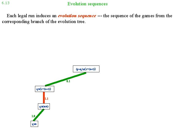
6. 13 Evolution sequences Each legal run induces an evolution sequence --- the sequence of the games from the corresponding branch of the evolution tree. (p⊔q) (r⊓(s⊔t)) 0. 1 q (r⊓(s⊔t)) 1. 1 q (s⊔t) 1. 0 q s

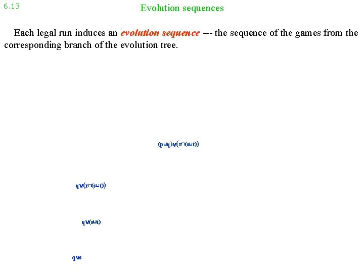
6. 13 Evolution sequences Each legal run induces an evolution sequence --- the sequence of the games from the corresponding branch of the evolution tree. (p⊔q) (r⊓(s⊔t)) q (s⊔t) q s

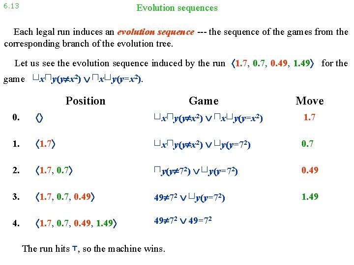
6. 13 Evolution sequences Each legal run induces an evolution sequence --- the sequence of the games from the corresponding branch of the evolution tree. Let us see the evolution sequence induced by the run 1. 7, 0. 49, 1. 49 for the game ⊔ x⊓ y(y x 2) ⊓ x⊔ y(y=x 2). Position Game Move 0. ⊔ x⊓ y(y x 2) ⊓ x⊔ y(y=x 2) 1. 7 ⊔ x⊓ y(y x 2) ⊔ y(y=72) 0. 7 2. 1. 7, 0. 7 ⊓ y(y 72) ⊔ y(y=72) 0. 49 3. 1. 7, 0. 49 72 ⊔ y(y=72) 1. 49 4. 1. 7, 0. 49, 1. 49 72 49=72 The run hits ⊤, so the machine wins.

6. 14 Evolution sequences for parallel quantification In a similar way can visualize Position 7. 1 Game x( Odd(x)⊔Odd(x)) x 6( Odd(x)⊔Odd(x)) Odd(7) x 8( Odd(x)⊔Odd(x)) Who is the winner? Move 0. 0 1. 1 2. 0 3. 1 4. 0 . . . - and -games as infinite - and -combinations. Machine Game x( Odd(x)⊔Odd(x)) Odd(0) x 1( Odd(x)⊔Odd(x)) Odd(0) Odd(1) x 2( Odd(x)⊔Odd(x)) Odd(0) Odd(1) Odd(2) x 3( Odd(x)⊔Odd(x)) Odd(0) Odd(1) Odd(2) Odd(3) x 4( Odd(x)⊔Odd(x)) . . . Who is the winner in this infinite run? Machine Are there any (legal) finite runs of this game won by the machine? No

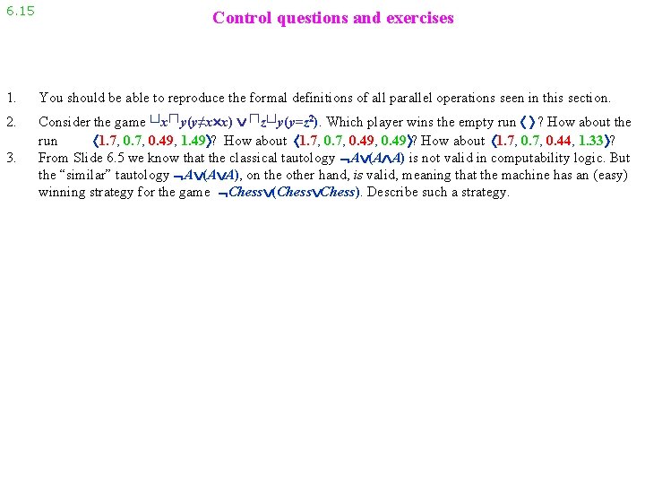
6. 15 Control questions and exercises 1. You should be able to reproduce the formal definitions of all parallel operations seen in this section. 2. Consider the game ⊔ x⊓ y(y≠x x) ⊓ z⊔ y(y=z 2). Which player wins the empty run ? How about the run 1. 7, 0. 49, 1. 49 ? How about 1. 7, 0. 49, 0. 49 ? How about 1. 7, 0. 44, 1. 33 ? From Slide 6. 5 we know that the classical tautology A (A A) is not valid in computability logic. But the “similar” tautology A (A A), on the other hand, is valid, meaning that the machine has an (easy) winning strategy for the game Chess (Chess). Describe such a strategy. 3.