Epidemiology Kept Simple Chapter 6 Incidence and Prevalence

Epidemiology Kept Simple Chapter 6 Incidence and Prevalence

Case Counts Prevalence count = no. of cases at particular time • Incidence count = no. of case onsets that accumulate over time •

Inadequacy of Case Counts • • Counts without context seldom useful in epi Convert count to ratios • Numerator – case count • Denominator – population “size”

Types of Ratios Used in Incidence and Prevalence • Rates ( ) • Change per unit time • Can be used to describe incidence • Proportions (p) • Mathematically distinct from rates • Can be used for incidence and prevalence • Odds (o) • Rarely used for descriptive purposes but are still used in some multivariate models

Types of Populations • • Closed = Cohorts Opened = Dynamic

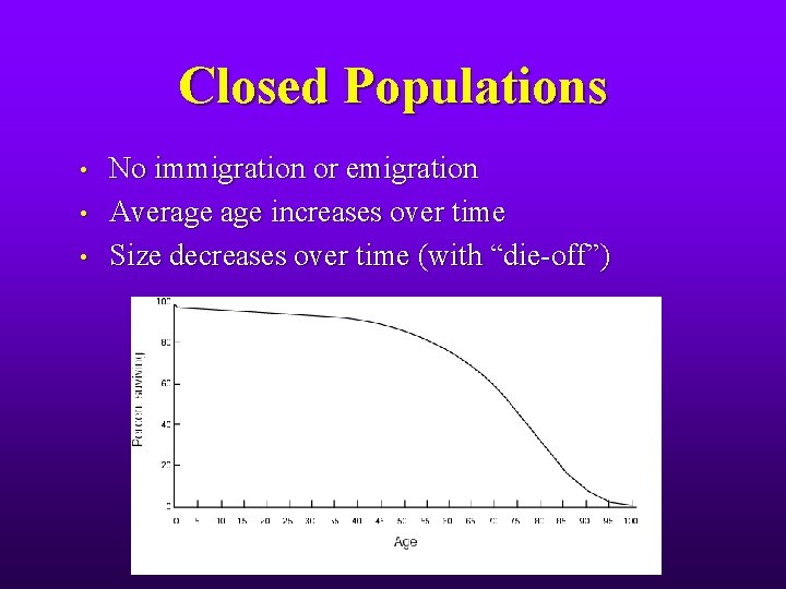
Closed Populations • • • No immigration or emigration Average increases over time Size decreases over time (with “die-off”)

Open Populations • Dynamics • • • Inflow = immigration & birth Outflow = emigration & death Average may increase, decrease, or stay the same Size may increase, decrease, or stay the same Stable (“stationary”) population = inflow balances outflow = maintains constant size and age structure over time

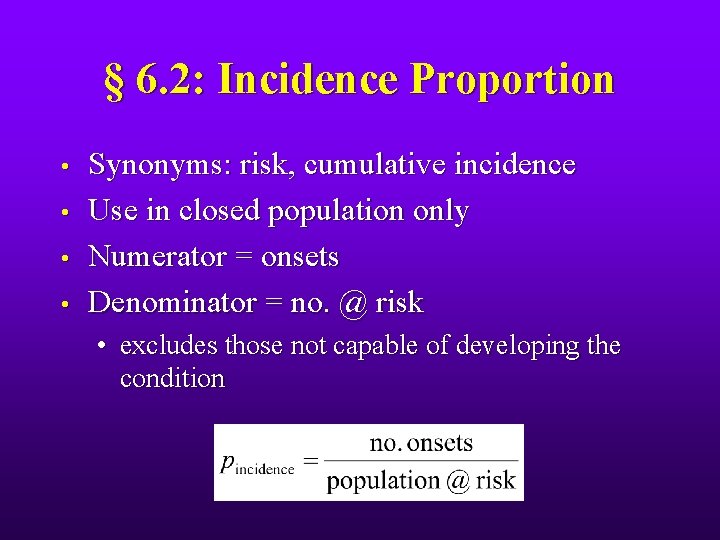
§ 6. 2: Incidence Proportion • • Synonyms: risk, cumulative incidence Use in closed population only Numerator = onsets Denominator = no. @ risk • excludes those not capable of developing the condition

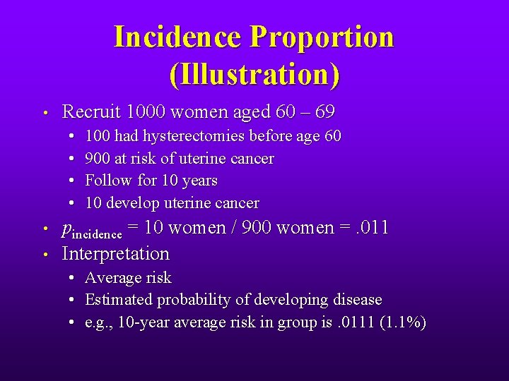
Incidence Proportion (Illustration) • Recruit 1000 women aged 60 – 69 • • • 100 had hysterectomies before age 60 900 at risk of uterine cancer Follow for 10 years 10 develop uterine cancer pincidence = 10 women / 900 women =. 011 Interpretation • • • Average risk Estimated probability of developing disease e. g. , 10 -year average risk in group is. 0111 (1. 1%)

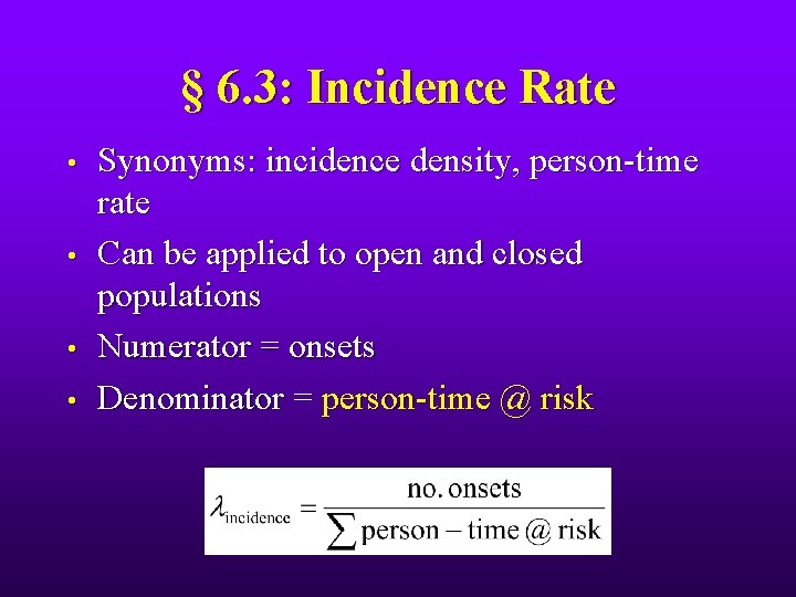
§ 6. 3: Incidence Rate • • Synonyms: incidence density, person-time rate Can be applied to open and closed populations Numerator = onsets Denominator = person-time @ risk

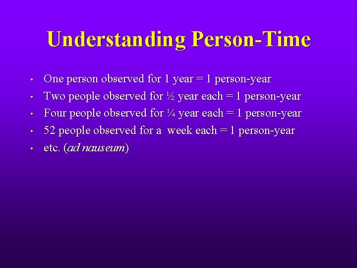
Understanding Person-Time • • • One person observed for 1 year = 1 person-year Two people observed for ½ year each = 1 person-year Four people observed for ¼ year each = 1 person-year 52 people observed for a week each = 1 person-year etc. (ad nauseum)

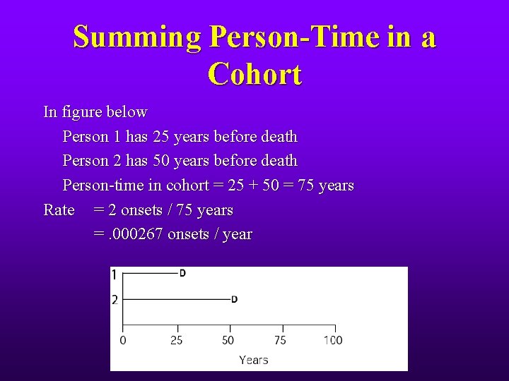
Summing Person-Time in a Cohort In figure below Person 1 has 25 years before death Person 2 has 50 years before death Person-time in cohort = 25 + 50 = 75 years Rate = 2 onsets / 75 years =. 000267 onsets / year

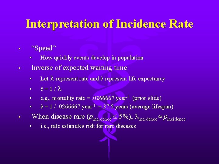
Interpretation of Incidence Rate • “Speed” • • Inverse of expected waiting time • Let represent rate and ê represent life expectancy • ê=1/ • • • How quickly events develop in population e. g. , mortality rate =. 0266667 year-1 (prior slide) ê = 1 /. 0266667 year-1 = 37. 5 years (average lifespan) When disease rare (pincidence 5%), incidence pincidence • i. e. , rate estimates risk for rare diseases

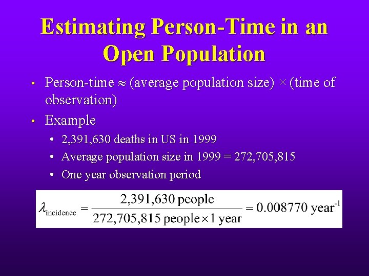
Estimating Person-Time in an Open Population • • Person-time (average population size) × (time of observation) Example • • • 2, 391, 630 deaths in US in 1999 Average population size in 1999 = 272, 705, 815 One year observation period

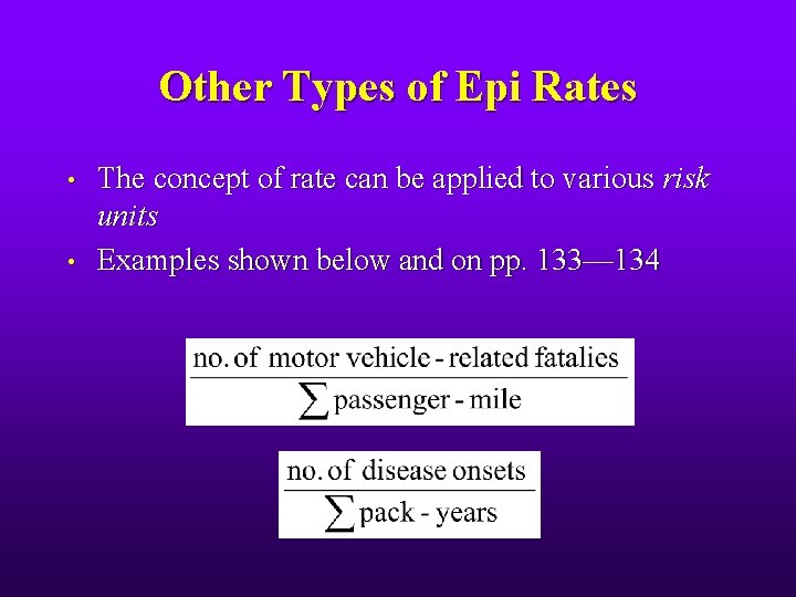
Other Types of Epi Rates • • The concept of rate can be applied to various risk units Examples shown below and on pp. 133— 134

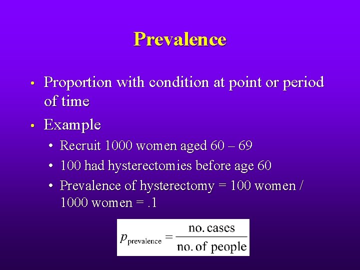
Prevalence • • Proportion with condition at point or period of time Example • • • Recruit 1000 women aged 60 – 69 100 had hysterectomies before age 60 Prevalence of hysterectomy = 100 women / 1000 women =. 1

Interpretation of Prevalence • • Prevalence = probability person selected at random has condition c. f. to incidence proportion (probability person selected at random will develop condition over stated time)

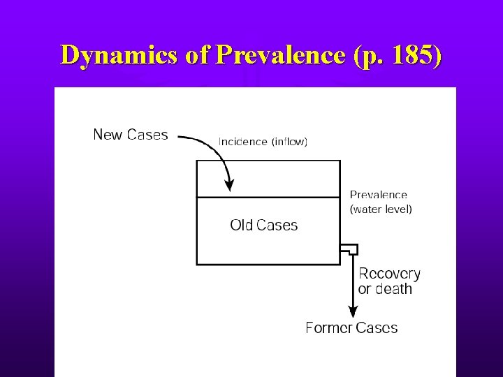
Dynamics of Prevalence (p. 185)

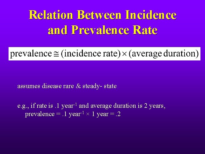
Relation Between Incidence and Prevalence Rate assumes disease rare & steady- state e. g. , if rate is. 1 year-1 and average duration is 2 years, prevalence =. 1 year-1 × 1 year =. 2

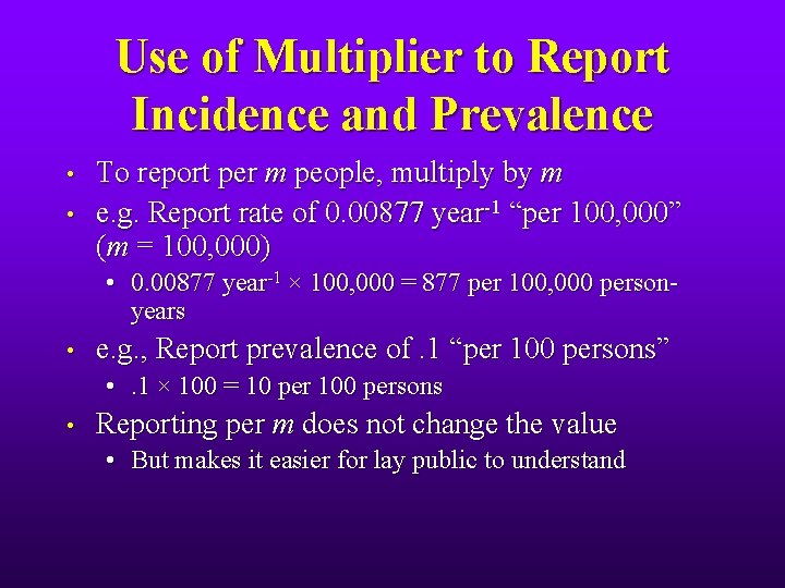
Use of Multiplier to Report Incidence and Prevalence • • To report per m people, multiply by m e. g. Report rate of 0. 00877 year-1 “per 100, 000” (m = 100, 000) • 0. 00877 year-1 × 100, 000 = 877 per 100, 000 personyears • e. g. , Report prevalence of. 1 “per 100 persons” • . 1 × 100 = 10 per 100 persons • Reporting per m does not change the value • But makes it easier for lay public to understand