Epi Info 2000 Main Menu Designing questionnaire Creating

Epi Info 2000: Main Menu Designing questionnaire Creating database, data entry Click. Tables (2 x 2, 2 xn), Sample size & power, Chi-square for trend. (See examples at the end of presentation. )

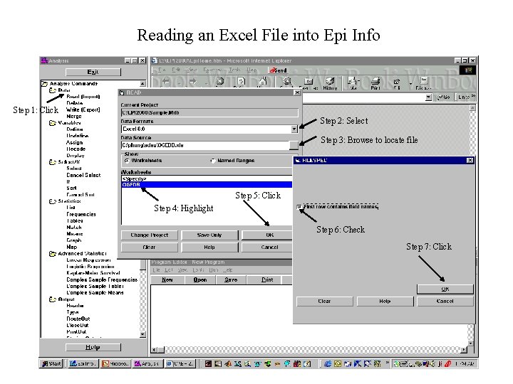
Reading an Excel File into Epi Info Step 1: Click Step 2: Select Step 3: Browse to locate file Step 5: Click Step 4: Highlight Step 6: Check Step 7: Click

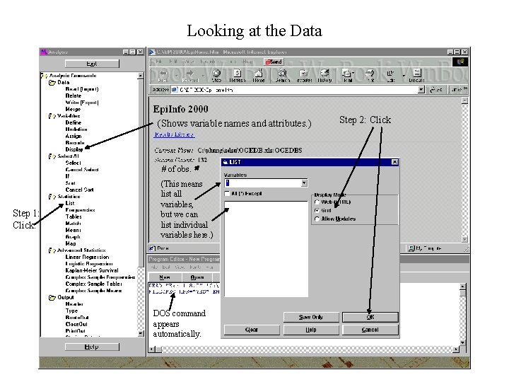
Looking at the Data (Shows variable names and attributes. ) # of obs. Step 1: Click. (This means list all variables, but we can list individual variables here. ) DOS command appears automatically. Step 2: Click

Looking at the Data– “Display” Output

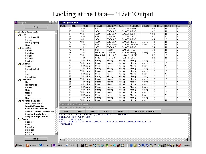
Looking at the Data— “List” Output

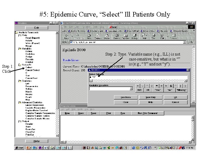
#5: Epidemic Curve, “Select” Ill Patients Only Step 1: Click Step 2: Type. Variable name (e. g. , ILL) is not case-sensitive, but what is in “” is (e. g. , “Y” and not “y”).

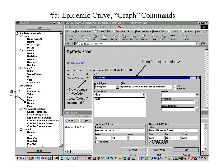
#5: Epidemic Curve, “Graph” Commands Step 2: Type as shown. Step 1: Click (Note change in # of obs. from “Select” command. ) date

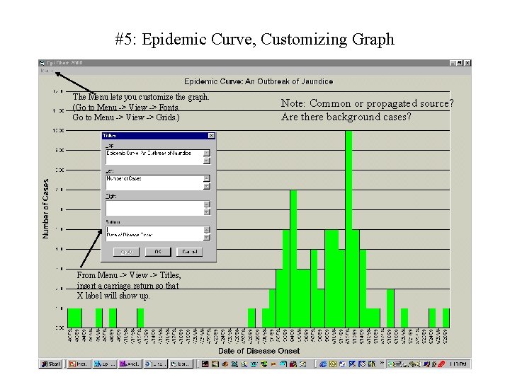
#5: Epidemic Curve, Customizing Graph The Menu lets you customize the graph. (Go to Menu -> View -> Fonts. Go to Menu -> View -> Grids. ) From Menu -> View -> Titles, insert a carriage return so that X label will show up. Note: Common or propagated source? Are there background cases?

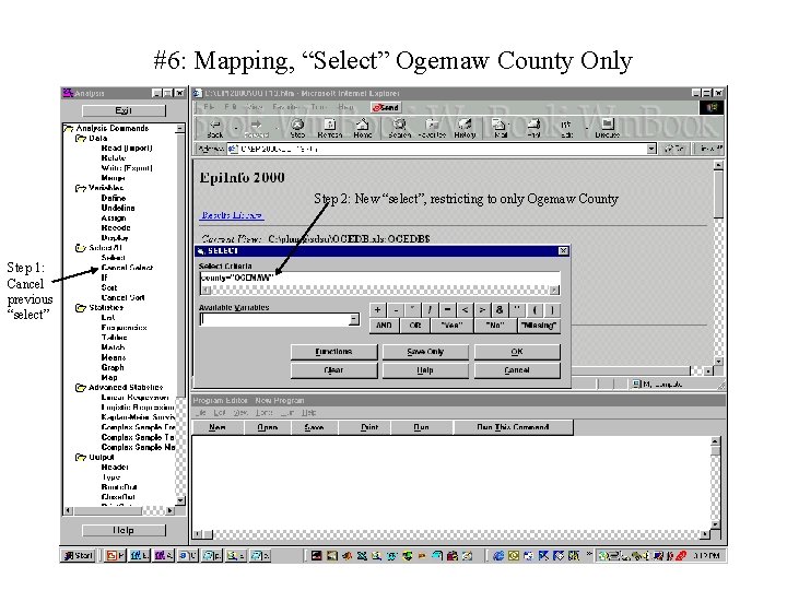
#6: Mapping, “Select” Ogemaw County Only Step 2: New “select”, restricting to only Ogemaw County Step 1: Cancel previous “select”

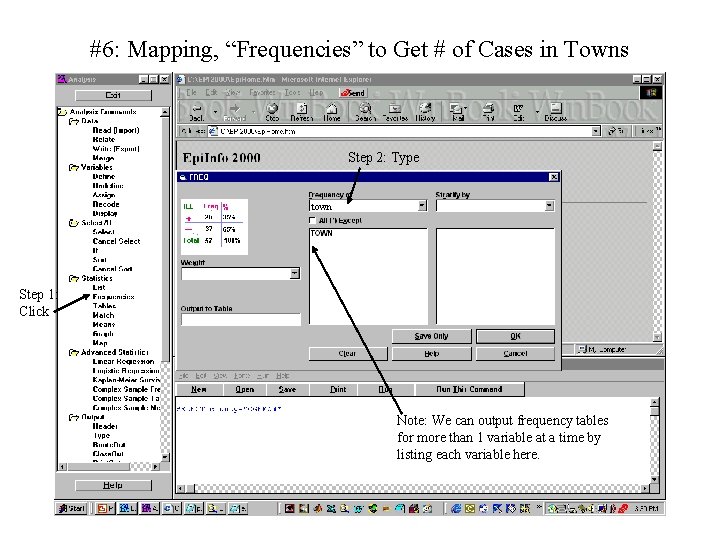
#6: Mapping, “Frequencies” to Get # of Cases in Towns Step 2: Type town Step 1: Click Note: We can output frequency tables for more than 1 variable at a time by listing each variable here.

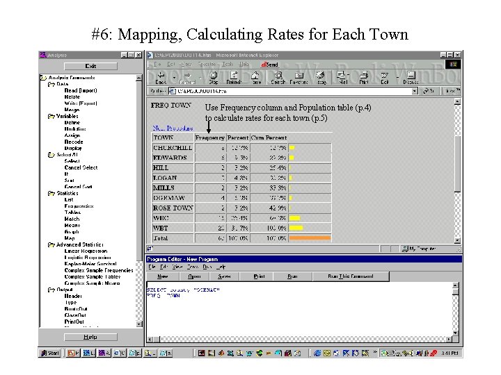
#6: Mapping, Calculating Rates for Each Town Use Frequency column and Population table (p. 4) to calculate rates for each town (p. 5)

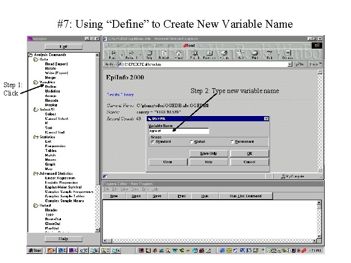
#7: Using “Define” to Create New Variable Name Step 1: Click Step 2: Type new variable name

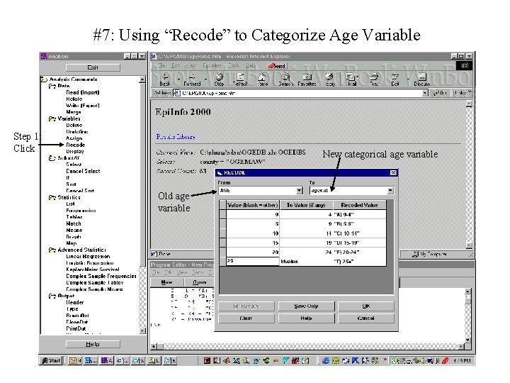
#7: Using “Recode” to Categorize Age Variable Step 1: Click New categorical age variable Old age variable

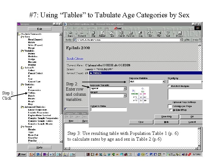
#7: Using “Tables” to Tabulate Age Categories by Sex Step 1: Click Step 2: Enter row and column variables. Step 3: Use resulting table with Population Table 1 (p. 6) to calculate rates by age and sex in Table 2 (p. 6)

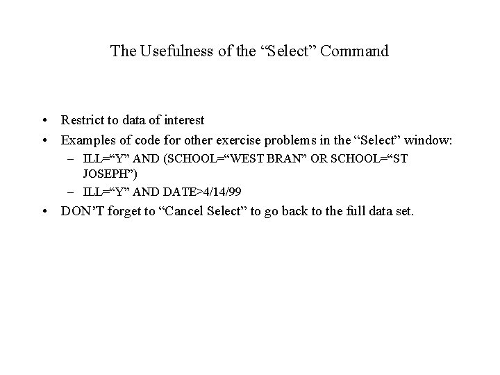
The Usefulness of the “Select” Command • Restrict to data of interest • Examples of code for other exercise problems in the “Select” window: – ILL=“Y” AND (SCHOOL=“WEST BRAN” OR SCHOOL=“ST JOSEPH”) – ILL=“Y” AND DATE>4/14/99 • DON’T forget to “Cancel Select” to go back to the full data set.

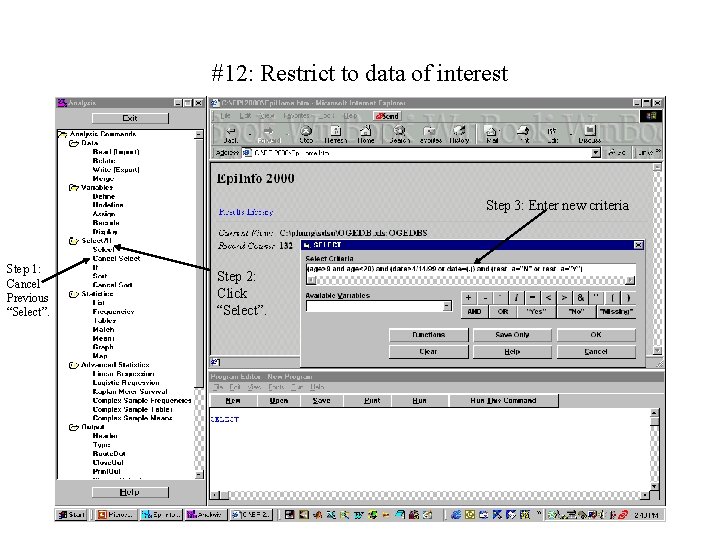
#12: Restrict to data of interest Step 3: Enter new criteria Step 1: Cancel Previous “Select”. Step 2: Click “Select”.

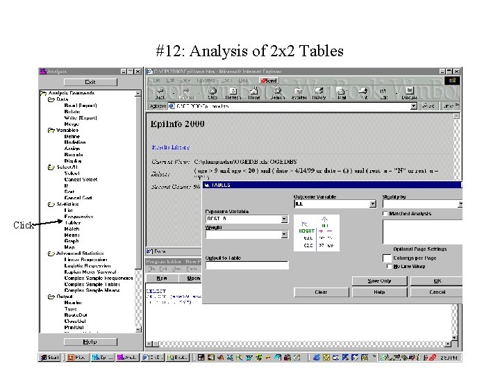
#12: Analysis of 2 x 2 Tables Click

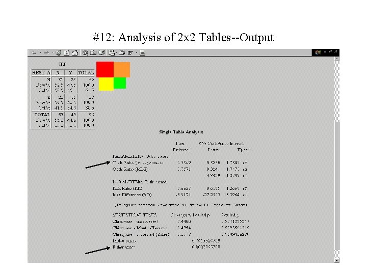
#12: Analysis of 2 x 2 Tables--Output

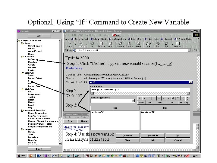
Optional: Using “If” Command to Create New Variable Step 1: Click “Define”. Type in new variable name (tw_do_g) Step 2: Click “If”. Step 3: Step 4: Use this new variable in an analysis of 2 x 2 table.

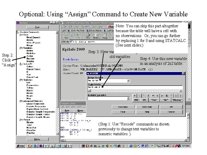
Optional: Using “Assign” Command to Create New Variable Note: You can skip this part altogether because the table will have a cell with no observations. Or, you can go further by replacing 1 for 0 and using STATCALC. (See next slides. ) Step 2: Click “Assign” Step 3: New variable = adding two old variables. Step 4: Use this new variable in an analysis of 2 x 2 table. (Step 1: Use “Recode” commands as shown previously to change text variables to numeric variables. )

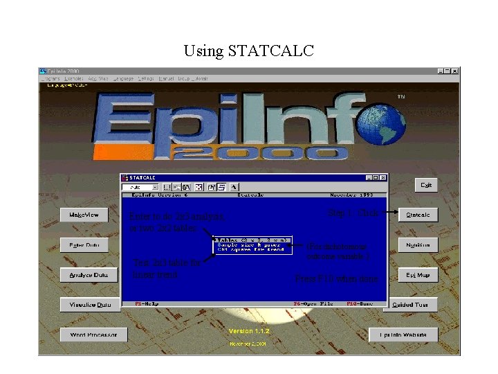
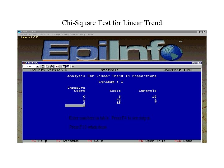
Using STATCALC Enter to do 2 x 3 analysis, or two 2 x 2 tables. Test 2 x 3 table for linear trend. Step 1: Click (For dichotomous outcome variable. ) Press F 10 when done.

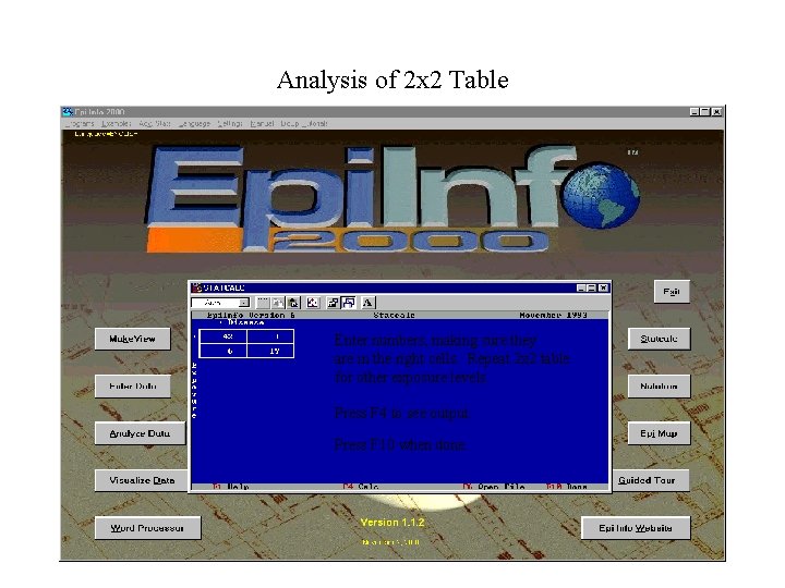
Analysis of 2 x 2 Table Enter numbers, making sure they are in the right cells. Repeat 2 x 2 table for other exposure levels. Press F 4 to see output. Press F 10 when done.

Chi-Square Test for Linear Trend Enter numbers in table. Press F 4 to see output. Press F 10 when done.

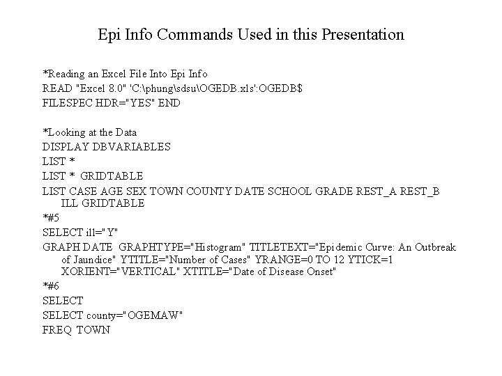
Epi Info Commands Used in this Presentation *Reading an Excel File Into Epi Info READ "Excel 8. 0" 'C: phungsdsuOGEDB. xls': OGEDB$ FILESPEC HDR="YES" END *Looking at the Data DISPLAY DBVARIABLES LIST * GRIDTABLE LIST CASE AGE SEX TOWN COUNTY DATE SCHOOL GRADE REST_A REST_B ILL GRIDTABLE *#5 SELECT ill="Y" GRAPH DATE GRAPHTYPE="Histogram" TITLETEXT="Epidemic Curve: An Outbreak of Jaundice" YTITLE="Number of Cases" YRANGE=0 TO 12 YTICK=1 XORIENT="VERTICAL" XTITLE="Date of Disease Onset" *#6 SELECT county="OGEMAW" FREQ TOWN

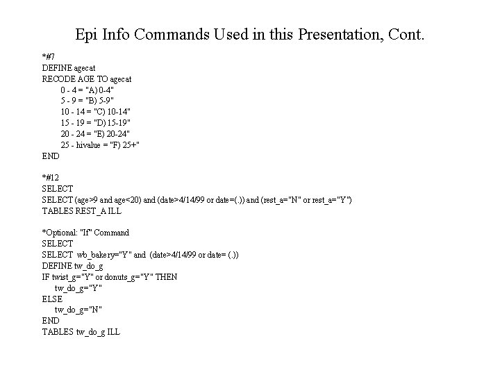
Epi Info Commands Used in this Presentation, Cont. *#7 DEFINE agecat RECODE AGE TO agecat 0 - 4 = "A) 0 -4" 5 - 9 = "B) 5 -9" 10 - 14 = "C) 10 -14" 15 - 19 = "D) 15 -19" 20 - 24 = "E) 20 -24" 25 - hivalue = "F) 25+" END *#12 SELECT (age>9 and age<20) and (date>4/14/99 or date=(. )) and (rest_a="N" or rest_a="Y") TABLES REST_A ILL *Optional: "If" Command SELECT wb_bakery="Y" and (date>4/14/99 or date= (. )) DEFINE tw_do_g IF twist_g="Y" or donuts_g="Y" THEN tw_do_g="Y" ELSE tw_do_g="N" END TABLES tw_do_g ILL

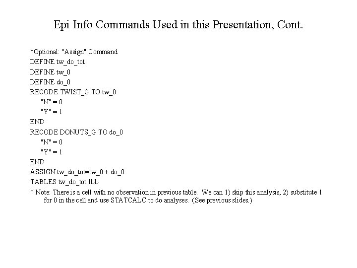
Epi Info Commands Used in this Presentation, Cont. *Optional: "Assign" Command DEFINE tw_do_tot DEFINE tw_0 DEFINE do_0 RECODE TWIST_G TO tw_0 "N" = 0 "Y" = 1 END RECODE DONUTS_G TO do_0 "N" = 0 "Y" = 1 END ASSIGN tw_do_tot=tw_0 + do_0 TABLES tw_do_tot ILL * Note: There is a cell with no observation in previous table. We can 1) skip this analysis, 2) substitute 1 for 0 in the cell and use STATCALC to do analyses. (See previous slides. )