EnvironmentalEconomic Performances in a Dynamic Setting Heterogeneous Slopes

Environmental-Economic Performances in a Dynamic Setting: Heterogeneous Slopes and Structural Breaks MASSIMILIANO MAZZANTI UNIVERSITY OF FERRARA CERIS CNR MILAN PALERMO, SEPTEMBER 12 TH 2012

Issues and Concepts Usefulness of Slope heterogeneity analysis in environmental economics & policy I will deal with examples under the umbrella of EKC and IPAT conceptual framework (structural change, decomposition analysis. . ) Rationales Econometric rationale (efficiency, correlation between units) Better food for thought for policy and management (specific firm, sector, country effects) More effective communication to non economist’s (the average coefficient problem. . )

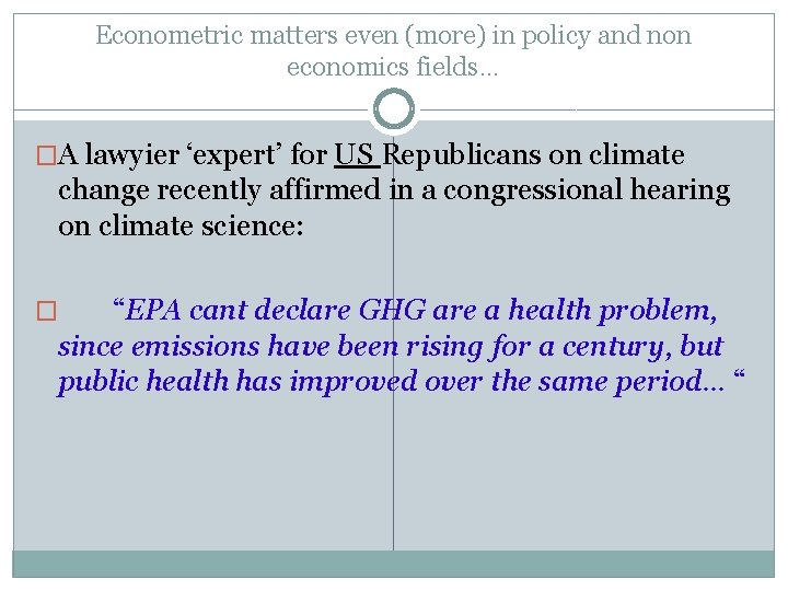
Econometric matters even (more) in policy and non economics fields… �A lawyier ‘expert’ for US Republicans on climate change recently affirmed in a congressional hearing on climate science: � “EPA cant declare GHG are a health problem, since emissions have been rising for a century, but public health has improved over the same period… “

Papers of Reference Nicolli F. Mazzanti M. Iafolla V. 2012, Waste Dynamics, Country Heterogeneity and European Environmental Policy Effectiveness, J of Environmental Policy and Planning, i-first Marin G. Mazzanti M. , 2012, The relationship between environmental and labour productivities, J of Evolutionary Economics, i-first Mazzanti M. Musolesi A. , The heterogeneity of Carbon Kuznets Curves for advanced countries. Comparing homogeneous, heterogeneous and shrinkage/Bayesian estimators 2012, Applied Economics forth. and FEEM nota di lavoro 2010

Slope heterogeneity in the environmental economics applied literature Recent advancements in EKC have focused on sub country and specific country heterogeneity in income -emission relationships Seminal paper by List and Gallett (1999), Ecological Economics, on CO 2 – income relationships at state level in the US Recent working paper by Martinez Espineira on Bird abundance and GDP growth in a panel of Canadian regions

We already tried to focus on specific homogeneous areas rather than OECD or full sample Source: Mazzanti, Musolesi and Zoboli, 2010, Applied Economics

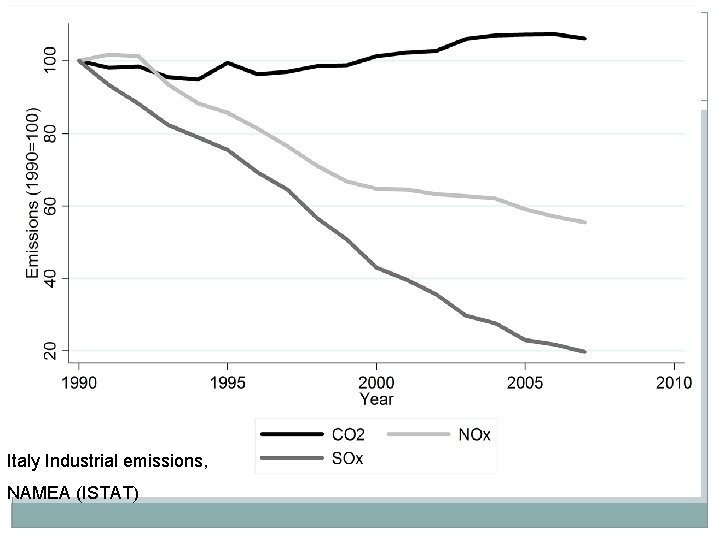
Italy Industrial emissions, NAMEA (ISTAT)

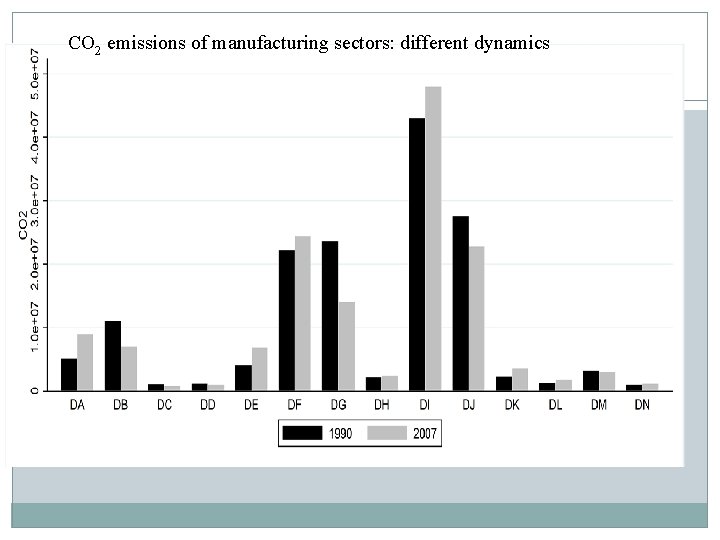
CO 2 emissions of manufacturing sectors: different dynamics

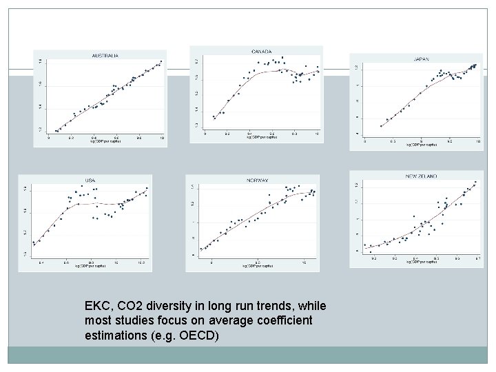
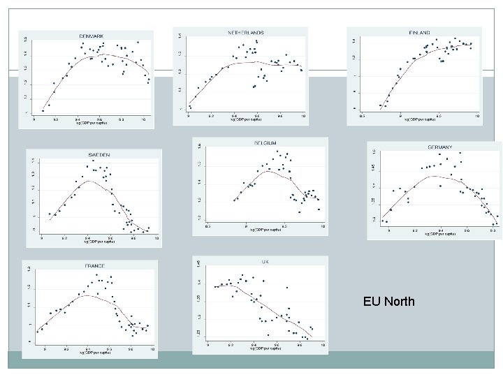
EKC, CO 2 diversity in long run trends, while most studies focus on average coefficient estimations (e. g. OECD)

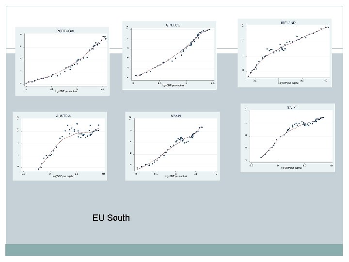
EU South

EU North

The way to deal with heterogeneity are many, some pragmatic some more technically refined We here hold attention on SUR – Seemingly Unrelated Regression - contexts

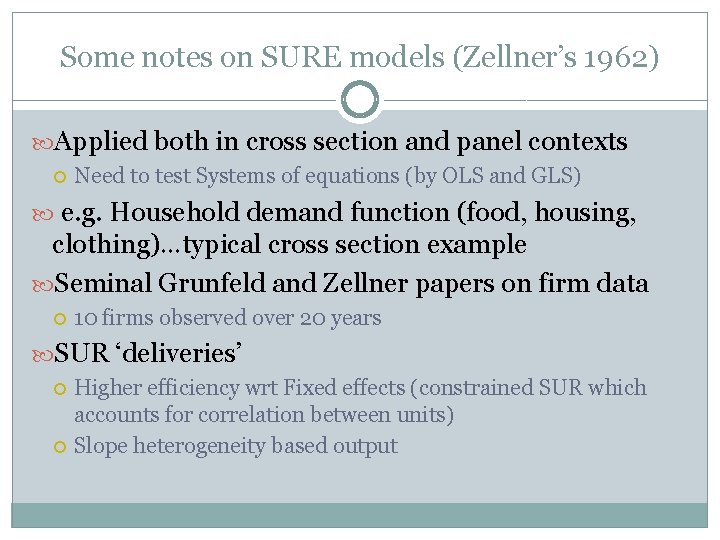
Some notes on SURE models (Zellner’s 1962) Applied both in cross section and panel contexts Need to test Systems of equations (by OLS and GLS) e. g. Household demand function (food, housing, clothing)…typical cross section example Seminal Grunfeld and Zellner papers on firm data 10 firms observed over 20 years SUR ‘deliveries’ Higher efficiency wrt Fixed effects (constrained SUR which accounts for correlation between units) Slope heterogeneity based output

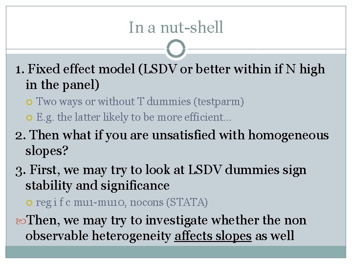
In a nut-shell 1. Fixed effect model (LSDV or better within if N high in the panel) Two ways or without T dummies (testparm) E. g. the latter likely to be more efficient… 2. Then what if you are unsatisfied with homogeneous slopes? 3. First, we may try to look at LSDV dummies sign stability and significance reg i f c mu 1 -mu 10, nocons (STATA) Then, we may try to investigate whether the non observable heterogeneity affects slopes as well

SUR In case we face a pretty long time series and a limited number of covariates, we can try to go further The issue is the contemporaneous correlation between cross sectional units E. g. systems of 10 equations with T=20 y 1 t = a 1 + b 1 x 1 t + 1 t y 2 t = a 2 + b 2 x 2 t + 2 t . . y 10 t = a 10 + b 10 x 10 t + 10 t

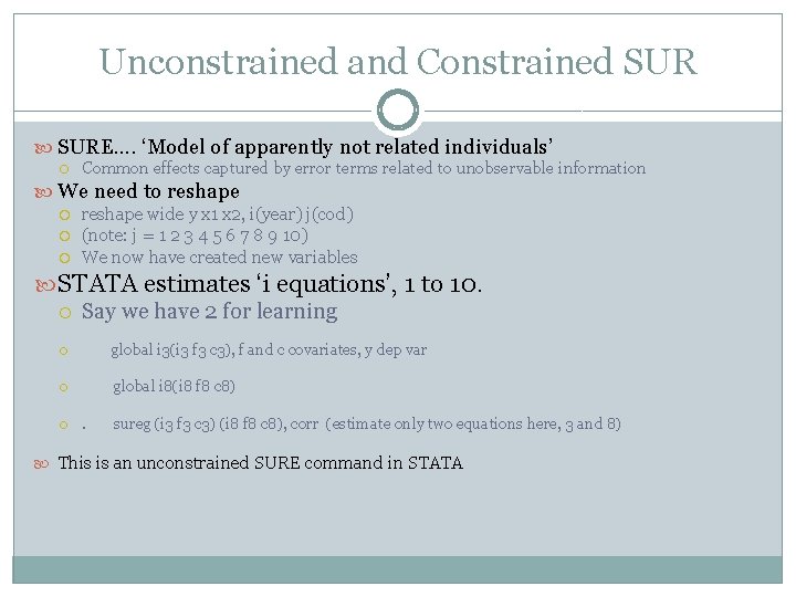
Unconstrained and Constrained SURE…. ‘Model of apparently not related individuals’ Common effects captured by error terms related to unobservable information We need to reshape wide y x 1 x 2, i(year) j(cod) (note: j = 1 2 3 4 5 6 7 8 9 10) We now have created new variables STATA estimates ‘i equations’, 1 to 10. Say we have 2 for learning global i 3(i 3 f 3 c 3), f and c covariates, y dep var global i 8(i 8 f 8 c 8) . sureg (i 3 f 3 c 3) (i 8 f 8 c 8), corr (estimate only two equations here, 3 and 8) This is an unconstrained SURE command in STATA

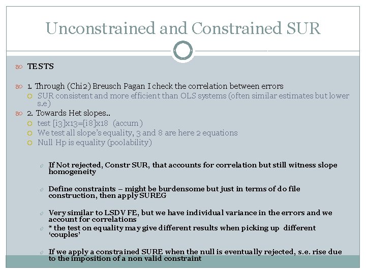
Unconstrained and Constrained SUR TESTS 1. Through (Chi 2) Breusch Pagan I check the correlation between errors SUR consistent and more efficient than OLS systems (often similar estimates but lower s. e) 2. Towards Het slopes. . test [i 3]x 13=[i 8]x 18 (accum) We test all slope’s equality, 3 and 8 are here 2 equations Null Hp is equality (poolability) If Not rejected, Constr SUR, that accounts for correlation but still witness slope homogeneity Define constraints – might be burdensome but just in terms of do file construction, then apply SUREG Very similar to LSDV FE, but we have individual variance in the errors and we account for correlations * the test on equality may give different results when picking up different ‘couples’ If we apply a constrained SURE when the null is eventually rejected, s. e. rise due to the imposition of a non valid constraint

Applications

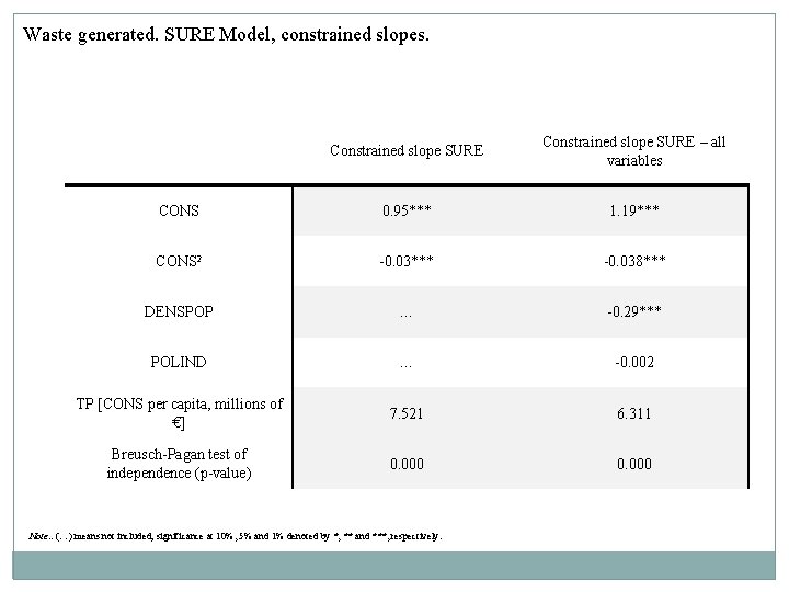
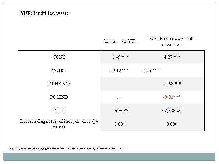
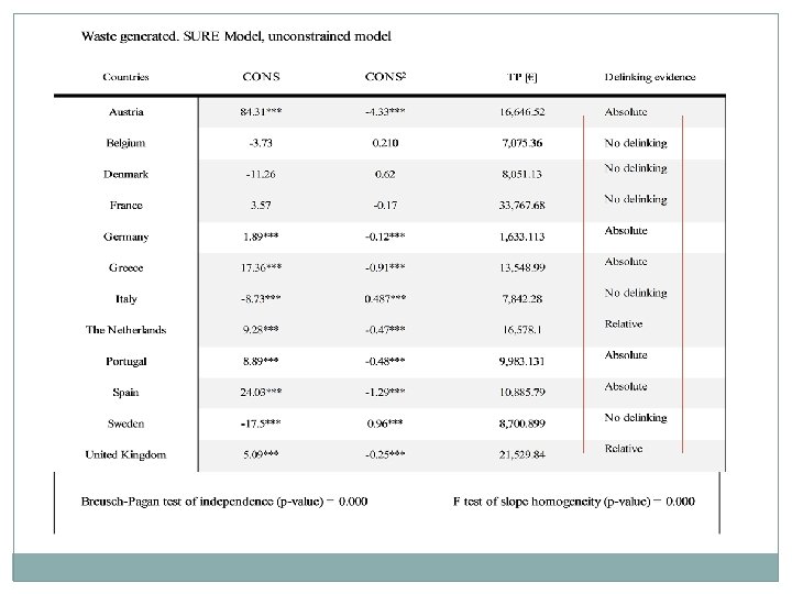
Nicolli et al. , JEPP 2012 Waste Kuznets curves in the EU EUROSTAT data for EU 15 over 1995 - 2008 Slope heterogeneity highlights various performances on decoupling

Waste generated. SURE Model, constrained slopes. Constrained slope SURE – all variables CONS 0. 95*** 1. 19*** CONS 2 -0. 03*** -0. 038*** DENSPOP … -0. 29*** POLIND … -0. 002 TP [CONS per capita, millions of €] 7. 521 6. 311 Breusch-Pagan test of independence (p-value) 0. 000 Note: . (…) means not included; significance at 10%, 5% and 1% denoted by *, ** and ***, respectively.

SUR: landfilled waste Constrained SUR – all covariates CONS 1. 49*** 4. 27*** CONS 2 -0. 10*** DENSPOP … -3. 68*** POLIND … -0. 82*** TP [€] 1, 659. 39 47, 328. 06 Breusch-Pagan test of independence (pvalue) 0. 000 Note: . (…) means not included; significance at 10%, 5% and 1% denoted by *, ** and ***, respectively. -0. 19***

Marin and Mazzanti, JEE, 2012 Environmental and labour productivity dynamics in Italy Sector based lens NAMEA (ISTAT) dataset on economic and environmental accounts: sector branches (e. g. Food, coke & refinery) over 1992 -2009 IPAT/EKC framework

SUR constrained estimates (manufacturing) - All emissions SUR [manuf] ln(CO 2/L) ln(NOx/L) ln(SOx/L) 2. 8517*** [0. 03] -3. 4261*** [0. 17] -11. 6507*** [0. 41] -0. 2745*** [0. 003] 0. 3455*** [0. 02] 1. 1463*** [0. 04] Stagnation 0. 0189*** [0. 001] 101. 91% -0. 2257*** [0. 02] 79. 79% -0. 8337*** [0. 05] 43. 45% Breusch-Pagan test of independence (Chi 2) 448. 746*** 376. 77*** 632. 504*** Test of aggregation bias (Chi 2) 16589. 74*** 19992. 81*** 3418. 68*** N*T 238 238 Period 1990 -2006 Turning point(s) 180. 3537*** [1. 94] 142. 3858*** [7. 83] 161. 0529*** [3. 52] Shape (VA/L) Inverted U shape ln(VA/L)2 s. e < FE case What hides behind aggregate shapes?

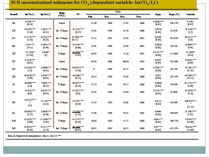
SUR unconstrained estimates for CO 2 (dependent variable: ln(CO 2/L) ) VA/L Branch ln(VA/L)2 Shape (VA/L) TP DA 2. 4189*** [0. 23] - Linear - 37. 99 1990 47. 95 DB 16. 2782*** [1. 46] -2. 2945*** [0. 21] Inv. U shape 34. 7145*** [0. 55] 23. 34 1990 DC 45. 1774*** [1. 53] -6. 5425*** [0. 22] Inv. U shape 31. 5834*** [0. 11] 25. 11 DD 15. 94*** [2. 41] -2. 2944*** [0. 36] Inv. U shape 32. 2564*** [0. 68] DE -25. 5248* [15. 32] 3. 6168* [2] U shape DF 0. 1429*** [0. 02] - DG 22. 4233*** [5. 2] DH Stagn. (%) Constant 2000 0. 1836*** [0. 05] 120. 15% 0. 4785 [0. 87] 34. 78 2000 -0. 0533 [0. 03] 94. 81% -19. 1502*** [2. 5] 1991 32. 58 2001 0. 0189 [0. 03] 101. 91% -69. 4115*** [2. 6] 22. 94 1990 32. 99 2001 -0. 0056 [0. 03] 99. 44% -18. 8895*** [4. 04] 34. 0792*** [5. 65] 40. 95 1990 51. 46 2001 0. 1121*** [0. 03] 111. 86% 54. 5399* [29. 3] Linear - 96. 92 2006 266. 04 1995 0. 0237 [0. 03] 102. 40% 12. 9344*** [0. 09] -2. 6966*** [0. 61] Inv. U shape 63. 9241*** [1. 46] 57 1990 82. 71 2004 -0. 1081*** [0. 03] 89. 75% -35. 1641*** [11. 01] 38. 0536*** [7. 09] -4. 9565*** [0. 94] Inv. U shape 46. 4664*** [0. 55] 40. 12 1990 49. 18 2006 0. 027 [0. 02] 102. 74% -63. 5661*** [13. 41] DI -38. 0085*** [2. 6] 5. 2095*** [0. 35] U shape 38. 3977*** [0. 32] 37. 13 1991 50. 17 2006 -0. 0098 [0. 02] 99. 02% 81. 1714*** [4. 86] DJ 42. 916*** [6. 9] -6. 0225*** [0. 94] Inv. U shape 35. 2677*** [0. 6] 32. 65 1990 43. 03 2002 -0. 1531*** [0. 04] 85. 80% -65. 9376*** [12. 6] DK 110. 5257** * [14] -14. 156*** [1. 81] Inv. U shape 49. 5927*** [0. 29] 42. 19 1993 50. 09 2000 -0. 0151 [0. 05] 98. 50% 206. 9535** * [27. 11] DL 30. 8633*** [2. 75] -3. 8026*** [0. 36] Inv. U shape 57. 8702*** [1. 42] 37. 38 1990 49. 21 2001 0. 0064 [0. 02] 100. 64% -54. 1085*** [5. 24] DM -85. 8531*** [7. 86] 11. 4303*** [1. 04] U shape 42. 7552*** [0. 19] 38. 02 1993 47. 11 2000 0. 0817** [0. 04] 108. 51% 170. 497*** [14. 86] DN 44. 0742*** [8. 46] -6. 1415*** [1. 22] Inv. U shape 36. 1696*** [0. 87] 28. 91 1991 36. 11 2000 0. 07*** [0. 02] 107. 25% -70. 8135*** [14. 68] Breusch-Pagan test of independence (Chi 2): 186. 514*** Min Year Max Year

�constrained SUR estimates for manufacturing confirm the result of FE estimates. It is worth noting that as expected SUR estimates are more efficient than FE, with lower standard error and ‘Stagnation’ structural break that becomes significant. �This gain in efficiency depends on the high correlation among the disturbances of the different sectors

�Unconstrained SUR estimates highlight an high degree of heterogeneity of the slopes across sectors, as confirmed by the test of the aggregation bias. �sectors that are robustly associated to absolute delinking are DG and DJ, both included in the EU ETS, and quite critical manufacturing sectors as far as pollution effects are concerned. �All other sectors show either linear (as DF, highly critical sector for GHG related environmental effects, with regional hot spots) or U shaped

false inference �The use of heterogeneous estimators can be motivated by the possible heterogeneity bias associated with the use of pooled estimators. As pointed out by Hsiao (2003), if the true model is characterised by heterogeneous intercepts and slopes, estimating a model with individual intercepts but common slopes could produce the false inference that the estimated relation is curvilinear.

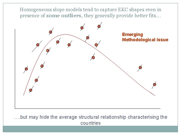
Homogeneous slope models tend to capture EKC shapes even in presence of some outliers, they generally provide better fits…. Emerging Methodological issue …. but may hide the average structural relationship characterising the countries

�WE defined 39 constraints, I am not showing the do file…

Mazzanti and Musolesi, 2010, 2012 Env. Kuznets. Curves Focus on advanced countries Looking at country / regions heterogeneity, income-time effects, structural breaks due to time related events

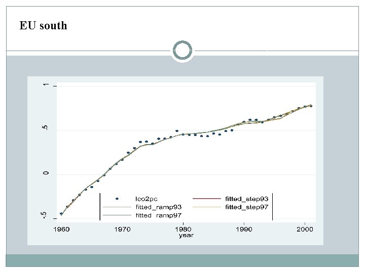
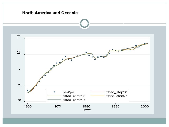
Structural breaks in a panel Environmental Policy shocks Oil shocks Those can be captured by the time related component of the income-environmental relationship. . Disentangle income and time effects… Further look at separated effects by country Back to the heterogeneity issue

EU south

North America and Oceania

EU North

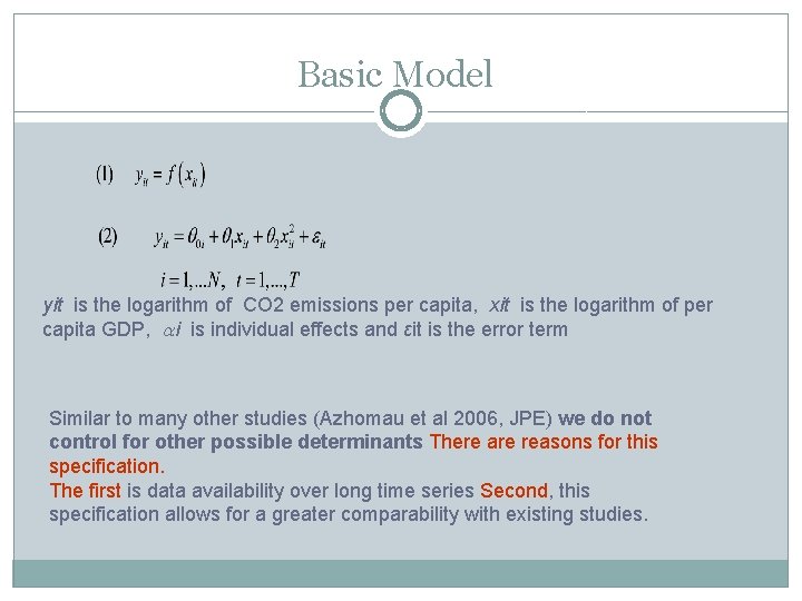
Basic Model yit is the logarithm of CO 2 emissions per capita, xit is the logarithm of per capita GDP, i is individual effects and εit is the error term Similar to many other studies (Azhomau et al 2006, JPE) we do not control for other possible determinants There are reasons for this specification. The first is data availability over long time series Second, this specification allows for a greater comparability with existing studies.

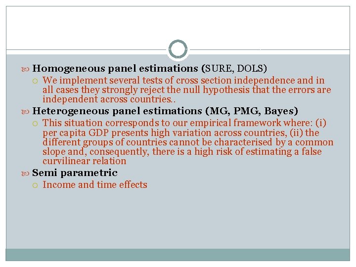
Homogeneous panel estimations (SURE, DOLS) We implement several tests of cross section independence and in all cases they strongly reject the null hypothesis that the errors are independent across countries. . Heterogeneous panel estimations (MG, PMG, Bayes) This situation corresponds to our empirical framework where: (i) per capita GDP presents high variation across countries, (ii) the different groups of countries cannot be characterised by a common slope and, consequently, there is a high risk of estimating a false curvilinear relation Semi parametric Income and time effects

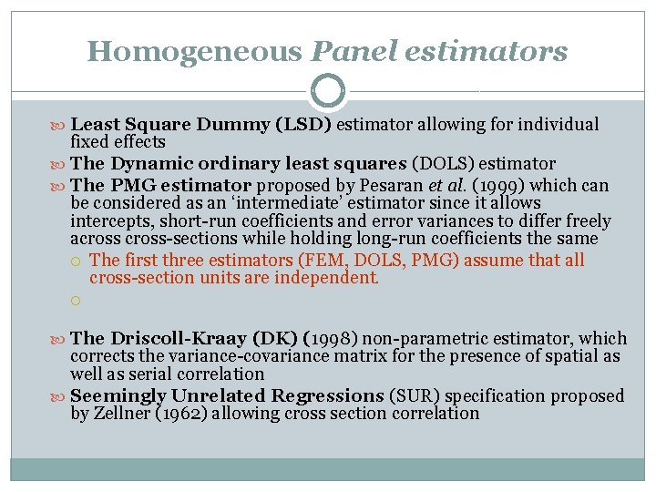
Homogeneous Panel estimators Least Square Dummy (LSD) estimator allowing for individual fixed effects The Dynamic ordinary least squares (DOLS) estimator The PMG estimator proposed by Pesaran et al. (1999) which can be considered as an ‘intermediate’ estimator since it allows intercepts, short-run coefficients and error variances to differ freely across-sections while holding long-run coefficients the same The first three estimators (FEM, DOLS, PMG) assume that all cross-section units are independent. The Driscoll-Kraay (DK) (1998) non-parametric estimator, which corrects the variance-covariance matrix for the presence of spatial as well as serial correlation Seemingly Unrelated Regressions (SUR) specification proposed by Zellner (1962) allowing cross section correlation

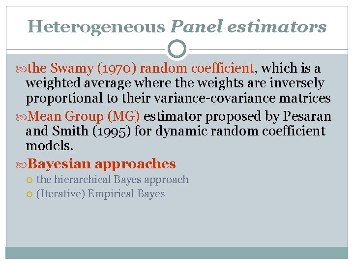
Heterogeneous Panel estimators the Swamy (1970) random coefficient, which is a weighted average where the weights are inversely proportional to their variance-covariance matrices Mean Group (MG) estimator proposed by Pesaran and Smith (1995) for dynamic random coefficient models. Bayesian approaches the hierarchical Bayes approach (Iterative) Empirical Bayes

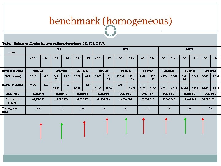
benchmark (homogeneous) Table 3 –Estimators allowing for cross sectional dependence: DK, SUR, DSUR DC SUR DSUR Model coef. Group of countries t-stat. Umbrella coef. t-stat. EU north coef. t-stat. EU south coef. t-stat. Umbrella coef. t-stat. EU north coef. t-stat. EU south GDPpc (linear) 3. 716 5. 97 16. 8 88 9. 96 2. 862 4. 87 3. 072 15. 1 33 15. 202 26. 1 65 2. 498 13. 2 87 3. 253 5. 667 10. 9 96 6. 062 3. 337 4. 654 GDPpc (quadratic) -0. 173 -5. 23 0. 890 -9. 89 0. 132 -4. 14 0. 138 12. 54 -0. 796 25. 67 0. 113 11. 30 0. 031 4. 613 0. 096 5. 979 0. 038 4. 211 EKC shape inverted U inverted U Inverted U inverted U Turning point ($1995) 46, 160. 715 13, 195. 623 51, 067. 782 68, 216. 025 14, 030. 586 63, 139. 216 87, 040. 245 14, 449. 242 out in out out in Turning point range inverted U 33, 796. 922 Out

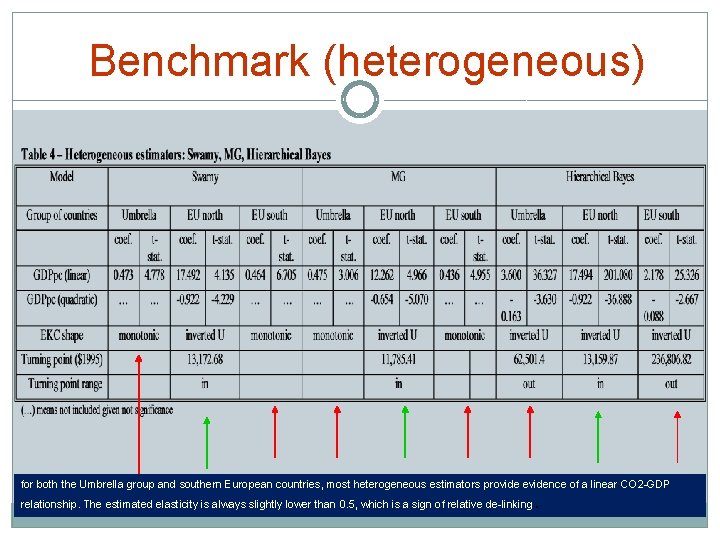
Benchmark (heterogeneous) for both the Umbrella group and southern European countries, most heterogeneous estimators provide evidence of a linear CO 2 -GDP relationship. The estimated elasticity is always slightly lower than 0. 5, which is a sign of relative de-linking .

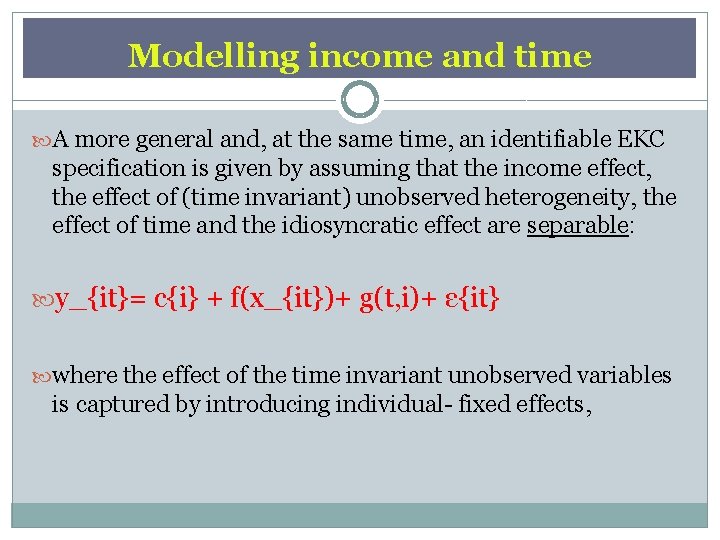
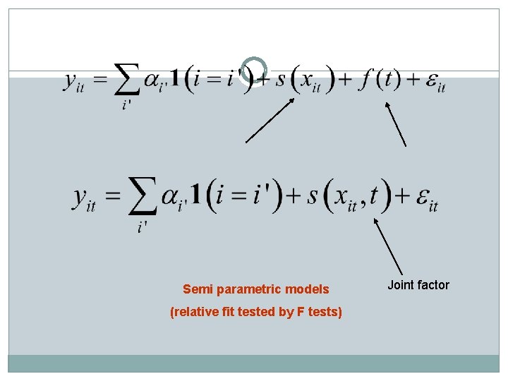
Modelling income and time A more general and, at the same time, an identifiable EKC specification is given by assuming that the income effect, the effect of (time invariant) unobserved heterogeneity, the effect of time and the idiosyncratic effect are separable: y_{it}= c{i} + f(x_{it})+ g(t, i)+ ε{it} where the effect of the time invariant unobserved variables is captured by introducing individual- fixed effects,

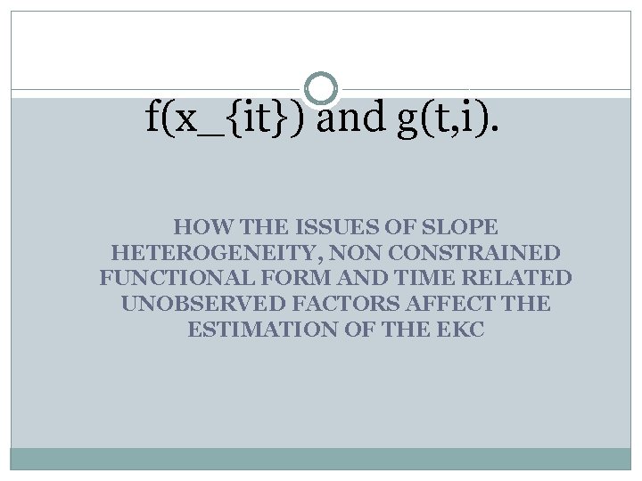
f(x_{it}) and g(t, i). HOW THE ISSUES OF SLOPE HETEROGENEITY, NON CONSTRAINED FUNCTIONAL FORM AND TIME RELATED UNOBSERVED FACTORS AFFECT THE ESTIMATION OF THE EKC

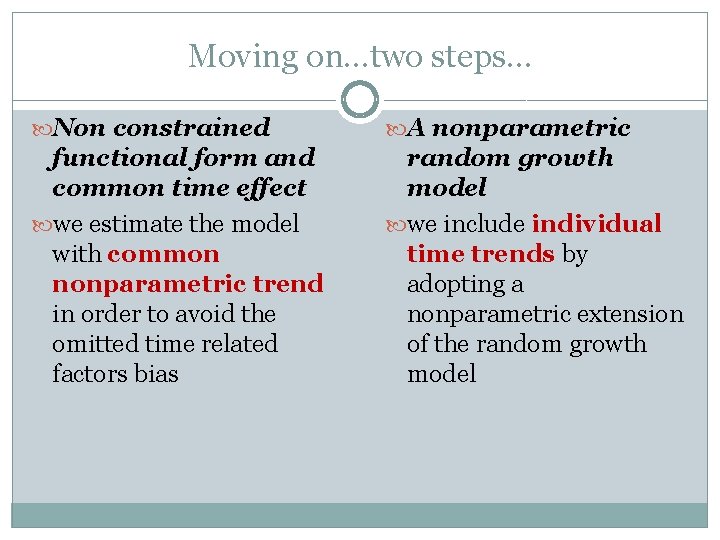
Moving on…two steps… Non constrained A nonparametric functional form and common time effect we estimate the model with common nonparametric trend in order to avoid the omitted time related factors bias random growth model we include individual time trends by adopting a nonparametric extension of the random growth model

Semi parametric models (relative fit tested by F tests) Joint factor

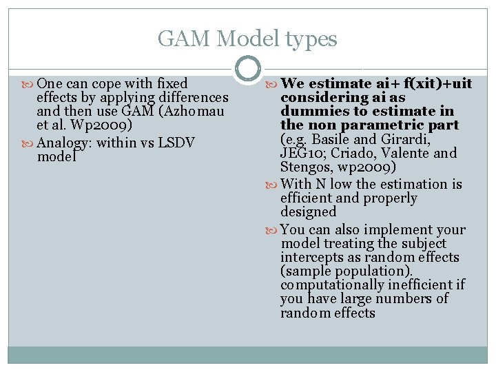
GAM Model types One can cope with fixed effects by applying differences and then use GAM (Azhomau et al. Wp 2009) Analogy: within vs LSDV model We estimate ai+ f(xit)+uit considering ai as dummies to estimate in the non parametric part (e. g. Basile and Girardi, JEG 10; Criado, Valente and Stengos, wp 2009) With N low the estimation is efficient and properly designed You can also implement your model treating the subject intercepts as random effects (sample population). computationally inefficient if you have large numbers of random effects

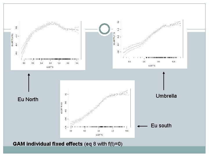
Eu North Umbrella Eu south GAM individual fixed effects (eq 8 with f(t)=0)

These results, thus, are on the one hand quite similar to those commented on above for parametric panel models, in terms of economic significance, but on the other hand at the same time highlight the limits of parametric formulations.

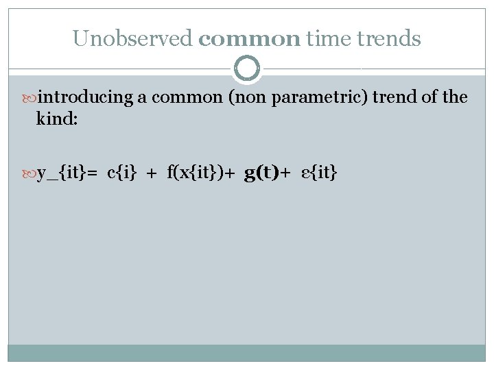
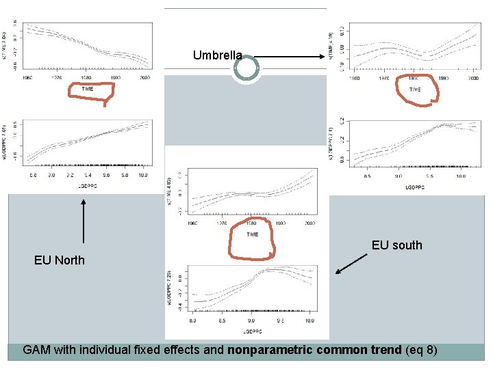
Unobserved common time trends introducing a common (non parametric) trend of the kind: y_{it}= c{i} + f(x{it})+ g(t)+ ε{it}

Umbrella EU south EU North GAM with individual fixed effects and nonparametric common trend (eq 8)

overall time evolution of per capita emissions is driven more by the unobserved common factors related to various time effects We believe that the issue is not what penalizes northern EU with regard to income related dynamics, but what has advantaged northern EU regarding the time related effects (over the all period, from the energy shock in the 70's 80's to the environmental policy era in the 90's).

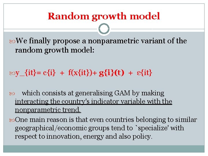
Random growth model We finally propose a nonparametric variant of the random growth model: y_{it}= c{i} + f(x{it})+ g{i}(t) + ε{it} which consists at generalising GAM by making interacting the country's indicator variable with the nonparametric trend. One main reason is that even countries belonging to similar geographical/economic groups tend to `specialize' with respect to innovation, energy and also policy.

1. Including individual time effects It is interesting to note that, beyond the economic policy's insights, including individual time effects is also important from a statistical point of view. Indeed, both the Akaike/Bayesian Information Criterion - AIC and BIC strongly support such specification against the common time effects specification (non linear) CO 2 -time shapes, inverted U North America, monotonic Oceania and South EU, Negative for EU NORTH

2. Individual time and income effects A more general specification can be obtained by considering both individual time effects and individual income effects it does improve very marginally upon the random growth - homogeneous income effect specification. Nevertheless, on the side of economic significance, we highlight that the only two countries showing an inverted U EKC / negative shape for both the income-carbon and CO 2 -time relationships are Sweden and Finland.

Main evidence Overall, the countries differ more on their carbon-time relation than on the carbonincome relation which is in almost all cases monotonic positive. Just a few Nordic countries show a bell curve in both income and time related factors.