Environmental time series 2008 Enviromatics 2008 Environmental time

Environmental time series Вонр. проф. д-р Александар Маркоски Технички факултет – Битола 2008 год. Enviromatics 2008 - Environmental time series 1

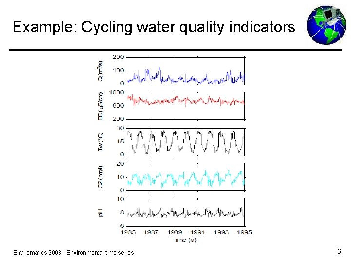
Introduction • Solving environmental problems or management tasks it is often necessary to analyse cycling (or periodic) processes. Cycling processes in ecology are natural. Such processes are caused mostly by natural external driving forces but also by natural and man-made internal driving forces. They lay out different time and frequency behaviour of ecological processes. • Mathematical equations have to describe either the time behaviour of an indicator (function of time t) or the frequency behaviour (function of frequency ω or cycles per time unit). Therefore, a description will be presented in the time domain in the frequency domain. • In next figure some examples of cycling processes with different periods and frequenciesare presented. Enviromatics 2008 - Environmental time series 2

Example: Cycling water quality indicators Enviromatics 2008 - Environmental time series 3

Environmental processes • The mathematical representation of environmental processes by trend functions is unsuitable to express high frequent changes of signals. Mostly, cycling (or periodic) ecological processes are caused by natural external driving forces. • On the other hand, aperiodic environmental processes are mainly influenced by artificial (man-made) external driving forces. Another distinction can be made by the ability to reproduce a time-varying process. • In the case of correct reproduction and forecast of a process it is called a deterministic one. • Otherwise it is called a non-deterministic or stochastic (random) process. Enviromatics 2008 - Environmental time series 4

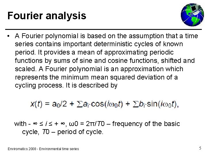
Fourier analysis • A Fourier polynomial is based on the assumption that a time series contains important deterministic cycles of known period. It provides a mean of approximating periodic functions by sums of sine and cosine functions, shifted and scaled. A Fourier polynomial is an approximation which represents the minimum mean squared deviation of a cycling process. It is described by with - ∞ ≤ i ≤ + ∞, ω0 = 2π/T 0 – frequency of the basic cycle, T 0 – period of cycle. Enviromatics 2008 - Environmental time series 5

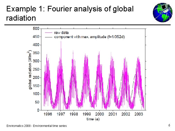
Example 1: Fourier analysis of global radiation Enviromatics 2008 - Environmental time series 6

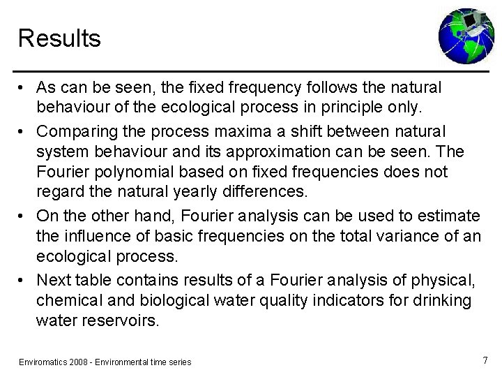
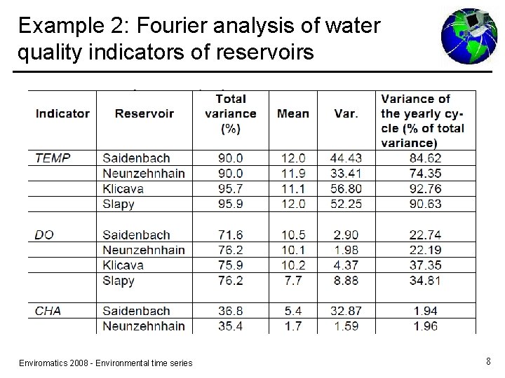
Results • As can be seen, the fixed frequency follows the natural behaviour of the ecological process in principle only. • Comparing the process maxima a shift between natural system behaviour and its approximation can be seen. The Fourier polynomial based on fixed frequencies does not regard the natural yearly differences. • On the other hand, Fourier analysis can be used to estimate the influence of basic frequencies on the total variance of an ecological process. • Next table contains results of a Fourier analysis of physical, chemical and biological water quality indicators for drinking water reservoirs. Enviromatics 2008 - Environmental time series 7

Example 2: Fourier analysis of water quality indicators of reservoirs Enviromatics 2008 - Environmental time series 8

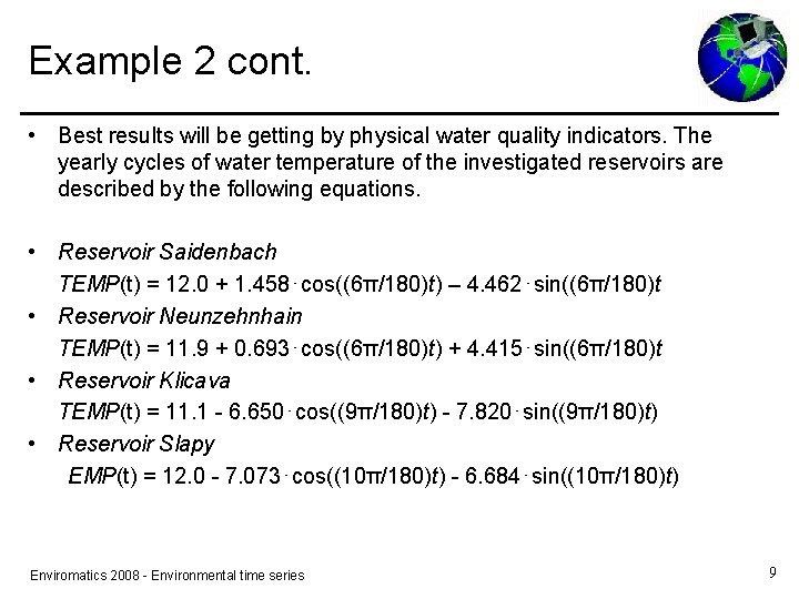
Example 2 cont. • Best results will be getting by physical water quality indicators. The yearly cycles of water temperature of the investigated reservoirs are described by the following equations. • Reservoir Saidenbach TEMP(t) = 12. 0 + 1. 458⋅cos((6π/180)t) – 4. 462⋅sin((6π/180)t • Reservoir Neunzehnhain TEMP(t) = 11. 9 + 0. 693⋅cos((6π/180)t) + 4. 415⋅sin((6π/180)t • Reservoir Klicava TEMP(t) = 11. 1 - 6. 650⋅cos((9π/180)t) - 7. 820⋅sin((9π/180)t) • Reservoir Slapy EMP(t) = 12. 0 - 7. 073⋅cos((10π/180)t) - 6. 684⋅sin((10π/180)t) Enviromatics 2008 - Environmental time series 9

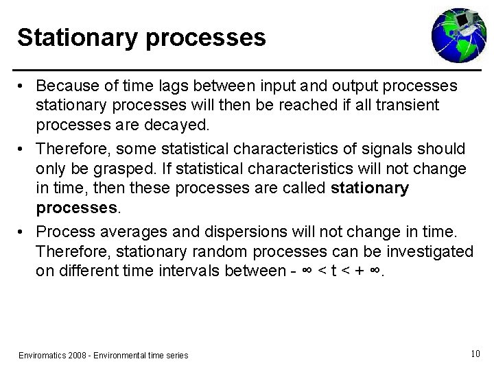
Stationary processes • Because of time lags between input and output processes stationary processes will then be reached if all transient processes are decayed. • Therefore, some statistical characteristics of signals should only be grasped. If statistical characteristics will not change in time, then these processes are called stationary processes. • Process averages and dispersions will not change in time. Therefore, stationary random processes can be investigated on different time intervals between - ∞ < t < + ∞. Enviromatics 2008 - Environmental time series 10

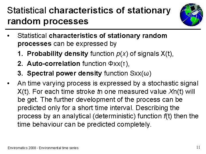
Statistical characteristics of stationary random processes • • Statistical characteristics of stationary random processes can be expressed by 1. Probability density function p(x) of signals X(t), 2. Auto-correlation function Φxx(τ), 3. Spectral power density function Sxx(ω) An time varying process is expressed by a stochastic signal X(t). For each time stroke tn one measured value Xn(t) will be get. The further development of the process can be predicted only for a short time interval. Describing the process by an analytical (deterministic) function f(t) then the time behaviour can be predicted completely. Enviromatics 2008 - Environmental time series 11

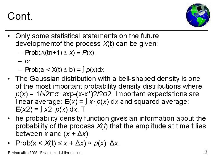
Cont. • Only some statistical statements on the future developmentof the process X(t) can be given: – Prob(X(tn+1) ≤ x) ≡ P(x), – or – Prob(a < X(t) ≤ b) = ∫ p(x)dx. • The Gaussian distribution with a bell-shaped density is one of the most important probability density distributions where p(x) = 1/√ 2πσ⋅exp-(x-x*)2/2σ2. Important expectations are linear average: E(x) = ∫ x⋅p(x) dx and squared average: E(x 2) = ∫ x 2⋅p(x) dx. T • he probability density function gives an information about the probability of the process X(t) that the amplitude at time t lies between x and (x + Δx): • Prob(x < X(t) ≤ x + Δx) ≈ p(x)⋅Δx. Enviromatics 2008 - Environmental time series 12

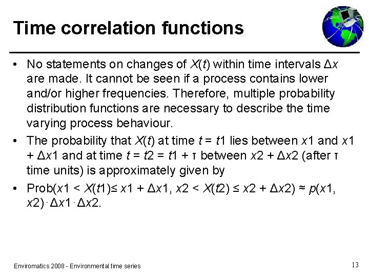
Time correlation functions • No statements on changes of X(t) within time intervals Δx are made. It cannot be seen if a process contains lower and/or higher frequencies. Therefore, multiple probability distribution functions are necessary to describe the time varying process behaviour. • The probability that X(t) at time t = t 1 lies between x 1 and x 1 + Δx 1 and at time t = t 2 = t 1 + τ between x 2 + Δx 2 (after τ time units) is approximately given by • Prob(x 1 < X(t 1)≤ x 1 + Δx 1, x 2 < X(t 2) ≤ x 2 + Δx 2) ≈ p(x 1, x 2)⋅Δx 1⋅Δx 2. Enviromatics 2008 - Environmental time series 13

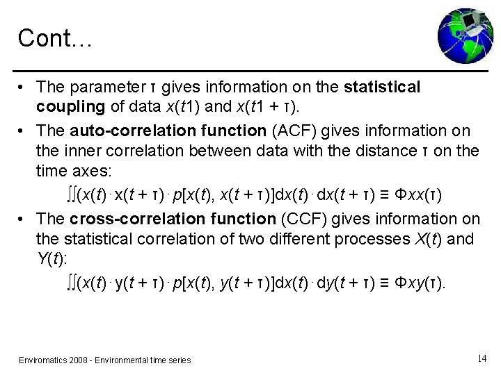
Cont… • The parameter τ gives information on the statistical coupling of data x(t 1) and x(t 1 + τ). • The auto-correlation function (ACF) gives information on the inner correlation between data with the distance τ on the time axes: ∫∫(x(t)⋅x(t + τ)⋅p[x(t), x(t + τ)]dx(t)⋅dx(t + τ) ≡ Φxx(τ) • The cross-correlation function (CCF) gives information on the statistical correlation of two different processes X(t) and Y(t): ∫∫(x(t)⋅y(t + τ)⋅p[x(t), y(t + τ)]dx(t)⋅dy(t + τ) ≡ Φxy(τ). Enviromatics 2008 - Environmental time series 14

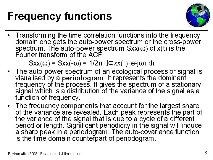
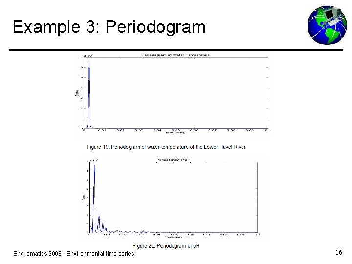
Frequency functions • Transforming the time correlation functions into the frequency domain one gets the auto-power spectrum or the cross-power spectrum. The auto-power spectrum Sxx(ω) of x(t) is the Fourier transform of the ACF: Sxx(ω) = Sxx(-ω) = 1/2π⋅∫Φxx(τ)⋅e-jωτ dτ. • The auto-power spectrum of an ecological process or signal is visualised by a periodogram. It represents the dominant frequency of the process. It gives the spectrum of a stationary signal which is a distribution of the variance of the signal as a function of frequency. • The frequency components that account for the largest share of the variance are revealed. Each peak represents the part of the variance of the signal that is due to a cycle of a different period or length. Significant periodicity in the signal will induce a sharp peak in a periodogram. The auto-covariance function is the time domain counterpart of periodogram. Enviromatics 2008 - Environmental time series 15

Example 3: Periodogram Enviromatics 2008 - Environmental time series 16

Coherency function • The cross-power spectrum Sxy(ω) of two stochastic ecological processes x(t) and y(t) is the Fourier transform of the CCF: • Sxy(ω) = 1/2π⋅∫Φxy(τ)⋅e-jωτ dτ It is a complex function. Coherency function • The coherency function Co(ω) is a measure of synchronicity of (two) signals. It is calculated on the base of periodograms of both signals by • Coxy(ω) = |Sxy(ω)|2/Sxx(ω)⋅Syy(ω), • where |Sxy(ω)| = √Re(Sxx(ω))2 + Re(Syy(ω))2 and for the phase shift between both signals ϕ(ω) = arc tan (Im(Sxy(ω))/Re(Sxy(ω))) is valid. • The limitation of CCF is considered by what is called a window function h(τ): • ~Sxy(ω) = 1/2π⋅∫Φxy(τ)⋅h(τ)⋅e-jωτ dτ = Sxy(α)⋅H(ω - α), • where H(ω) is the Fourier transform of h(τ) which distorts Sxy(ω) to ~Sxy(ω). Enviromatics 2008 - Environmental time series 17

Environmental time series The End Enviromatics 2008 - Environmental time series 18