Environmental Remote Sensing GEOG 2021 Lecture 8 Orbits

Environmental Remote Sensing GEOG 2021 Lecture 8 Orbits, scale and trade-offs, revision

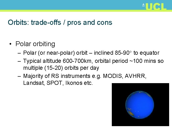
Orbits: trade-offs / pros and cons • Polar orbiting – Polar (or near-polar) orbit – inclined 85 -90 to equator – Typical altitude 600 -700 km, orbital period ~100 mins so multiple (15 -20) orbits per day – Majority of RS instruments e. g. MODIS, AVHRR, Landsat, SPOT, Ikonos etc.

Orbits and trade-offs: polar • Advantages – Higher spatial resolution (<m to few km), depending on instrument and swath width – Global coverage due to combination of orbit path and rotation of Earth • Disadvantages – Takes time to come back to point on surface e. g. 1 or 2 days for MODIS, 16 days for Landsat

Orbits: trade-offs / pros and cons • Geostationary – Orbit over equator, with orbit period (by definition) of 24 hours – Always in same place over surface – 36, 000 km altitude i. e. MUCH further away then polar

Orbits and trade-offs: Geostationary • Advantages – Always look at same part of Earth – Rapid repeat time (as fast as you like) e. g. Meteosat every 15 minutes - ideal for weather monitoring/forecasting • Disadvantages – Much higher (36000 km) altitude means lower resolution – Not global coverage – see same side of Earth

Orbits and trade-offs: Geostationary METEOSAT 2 nd Gen (MSG) (geostationary orbit) 1 km (equator) to 3 km (worse with latitude) Views of whole Earth disk every 15 mins 30+ years METEOSAT data MSG-2 image of Northern Europe “Mostly cloud free”

Remember, we always have trade-offs in space, time, wavelength etc. – determined by application • Global coverage means broad swaths, moderate-to-low resolution – Accept low spatial detail for global coverage & rapid revisit times – Land cover change, deforestation, vegetation dynamics, surface reflectance, ocean and atmospheric circulation, global carbon & hydrological cycle – E. g. MODIS (Terra, Aqua) (near-polar orbit) • 250 m to 1 km, 7 bands across visible + NIR, swath width ~2400 km, repeat 1 -2 days – MERIS (near-polar orbit) • ~300 m, 15 bands across visible + NIR, swath width ~1100 km, repeat time hours to days

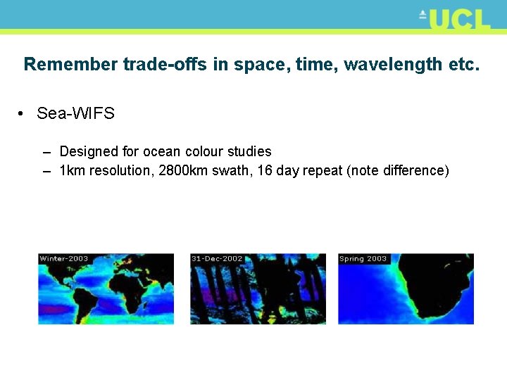
Remember trade-offs in space, time, wavelength etc. • Sea-WIFS – Designed for ocean colour studies – 1 km resolution, 2800 km swath, 16 day repeat (note difference)

Remember trade-offs in space, time, wavelength etc. MERIS image of Californian fires October 2007

Remember trade-offs in space, time, wavelength etc. • Local to regional – Requires much higher spatial resolution (< 100 m) – So typically, narrower swaths (10 s to 100 s km) and longer repeat times (weeks to months) – E. g. Landsat (polar orbit) • 28 m spatial, 7 bands, swath ~185 km, repeat time nominally 16 days BUT optical, so clouds can be big problem – E. g. Ikonos (polar orbit • 0. 5 m spatial, 4 bands, swath only 11 km, so requires dedicated targeting

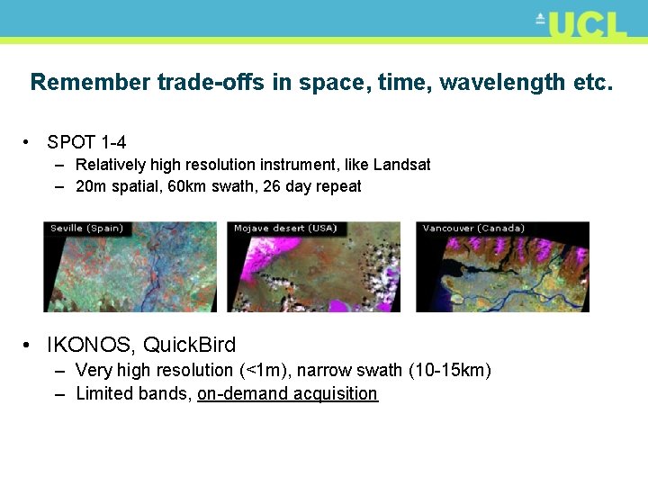
Remember trade-offs in space, time, wavelength etc. • SPOT 1 -4 – Relatively high resolution instrument, like Landsat – 20 m spatial, 60 km swath, 26 day repeat • IKONOS, Quick. Bird – Very high resolution (<1 m), narrow swath (10 -15 km) – Limited bands, on-demand acquisition

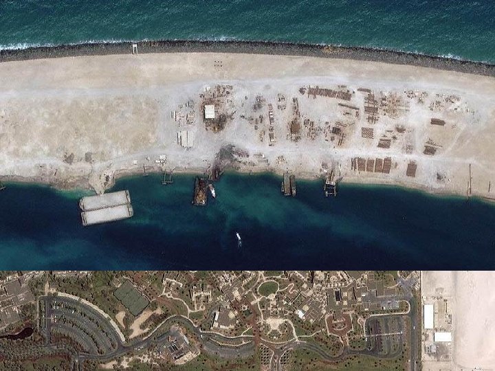
A changing world: Earth Palm Jumeirah, UAE Images courtesy Geo. EYE/SIME

Summary • Instrument characteristics determined by application – How often do we need data, at what spatial and spectral resolution? – Can we combine observations? ? – E. g. optical AND microwave? LIDAR? Polar and geostationary orbits? Constellations?

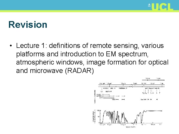
Revision • Lecture 1: definitions of remote sensing, various platforms and introduction to EM spectrum, atmospheric windows, image formation for optical and microwave (RADAR)

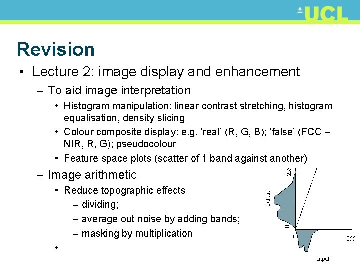
Revision • Lecture 2: image display and enhancement – To aid image interpretation 255 • Histogram manipulation: linear contrast stretching, histogram equalisation, density slicing • Colour composite display: e. g. ‘real’ (R, G, B); ‘false’ (FCC – NIR, R, G); pseudocolour • Feature space plots (scatter of 1 band against another) 0 • Reduce topographic effects – dividing; – average out noise by adding bands; – masking by multiplication • output – Image arithmetic 0 255 input

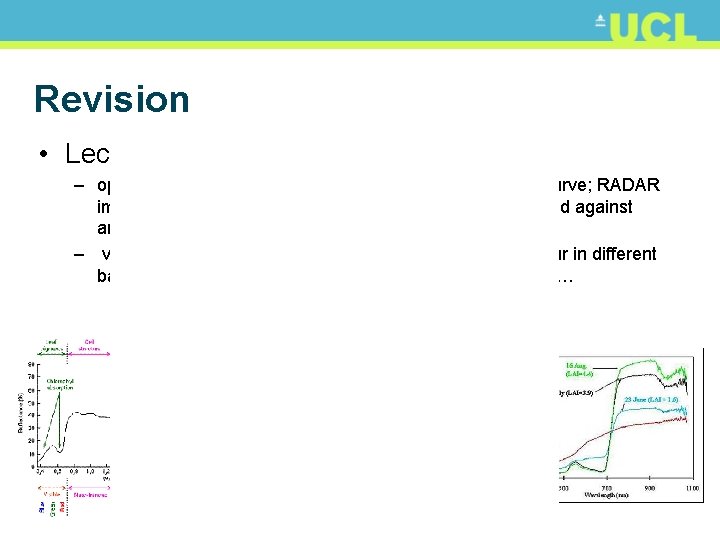
Revision • Lecture 3: spectral information – optical, vegetation examples – characteristic vegetation curve; RADAR image characteristics, spectral curves, scatter plots (1 band against another) – vegetation indices exploit contrast in reflectance behaviour in different bands e. g. NDVI (NIR-R/)(NIR+R). Perpendicular, parallel…

Revision • Lecture 4: classification – Producing thematic information from raster data – Supervised (min. distance, parallelepiped, max likelihood etc. ) – Unsupervised (ISODATA) – iterative clustering – Accuracy assessment: confusion matrix • Producers accuracy: how many pixels I know are X are correctly classified as X? Errors of omission • Users accuracy: how many pixels in class Y that I know don’t belong there? Errors of comission

Revision • L 5: spatial operators, convolution filtering – 1 D examples e. g. mean filter [1, 1, 1] smooths out (low pass filter) • 1 st differential (gradient) [-1, 0, 1] - detects edges (high pass filter) • 2 nd differential (2 nd order gradient) [1, -2, 1] detects edges of edges (high pass) – Applications: • Low-pass filter to smooth RADAR speckle • High-pass to detect edges of field boundaries, or directions of edges e. g. roads in an image; • Or slope (gradient) and aspect (direction) e. g. apply 1 in x direction and 1 in y direction – result direction vector = aspect; size = steepness (slope)

Revision • L 6: Modelling 1 - types of model – Empirical – based on observations; simple, quick BUT give no understanding of system, limited in application e. g. linear model of biomass as function of NDVI – Physical - represent underlying physical system; typically more complex, harder to invert BUT parameters have physical meaning e. g. complex hydrological model

Revision • Lecture 7: Modelling 2 – Simple (but physical) population model – Empirical regression model, best fit i. e. find line which gives minimum error (root mean square error, RMSE) – Forward modelling • Provide parameter values, use model to predict state of system - useful for understanding system behaviour e. g. backscatter = f(LAI), can predict backscatter for given LAI in forward direction – Inverse modelling • Measure system, and invert parameters of interest e. g. LAI = f 1(backscatter) • Today – spatial coverage: local v global?

References • Global land cover & land cover change • • http: //glcf. umiacs. umd. edu/services/landcoverchange/ B. L. Turner, II*, , Eric F. Lambin , and Anette Reenberg The emergence of land change science for global environmental change and sustainability, PNAS 2007, http: //www. pnas. org/cgi/content/full/104/52/20666 http: //lcluc. umd. edu/ http: //visibleearth. nasa. gov/view_rec. php? id=3446 • Deforestation • http: //visibleearth. nasa. gov/view_set. php? category. ID=582