Environmental Modeling Advanced Weighting of GIS Layers 2

Environmental Modeling Advanced Weighting of GIS Layers (2)

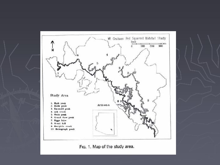
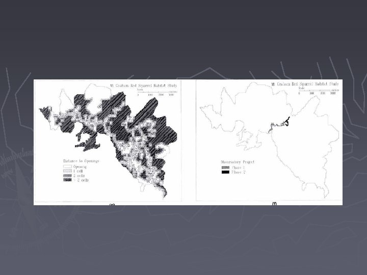
1. Issue ► Modeling the habitat of red squirrel in the Mt. Graham area ► Red squirrel prefer a shaded and humid environment and feed on pine cones, that are offered by Mt. Graham ► The issue is whether the construction of an astronomy observatory will affect the habitat Pereira, J. M. C. , and R. M. Itami, 1991. GIS-based habitat modeling using logistic multiple regression: a study of the Mt. Graham Red Squirrel. Photogrammetric Engineering and Remote Sensing, 57(11): 1475 -1486.

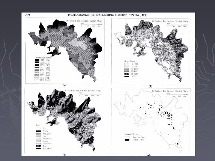
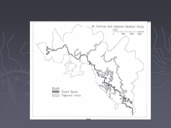
2. Factors a. Topography: b. Vegetation: Elevation Land cover Slope Canopy closure Aspect (e-w) Food productivity Aspect (n-s) Tree diameter c. Distance to openness (canopy closure and roads)

3. Spatial Sampling ► The 200 presence sites are observed in the field The 200 absence sites can be randomly generated using Hawth’s tool ► OR systematically sampled every nth cell, Then n=? ►

At each of the 400 locations, collect both dependent and the independent variables

3. Spatial Sampling. . ► Moran’s ► I Cij = 1, if xi and xj are adjacent, Cij=0 otherwise

3. Spatial Sampling. . Moran’s I. . ► I = 1 indicates a positive spatial autocorrelation ► I = -1 indicates a negative spatial autocorrelation ► I = 0 indicates a random spatial pattern

3. Spatial Sampling. . Ileft = 0. 94, Imiddle = -1, Iright = 0. 168

3. Spatial Sampling. . ► The spatial lag can be any value, e. g. 1, 2, 3, 4, …. ► When the lag distance increases, the pairs of i and j locations are further apart ► The I value decreases with an increasing lag distance, indicating increasing differences between values at i and j locations

3. Spatial Sampling. . ► Moran’s I is applied to each variable lag = 1, 2, 3, … 7 ► When lag = 1, I is close to 1 ► When lag= 7, I = 0. 16 – 0. 34 among the ind variables ► Every 7 th cell is selected ► 259 absence cells, compatible to the 212 presence cells ►

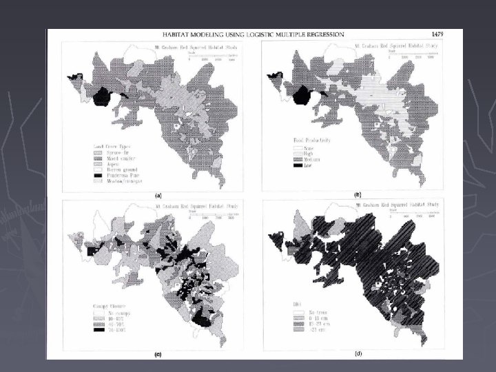
independent variables ► Independent variables (14) the continuous variables (1 -5, ratio data) 1. Elevation 2. slope 3. aspect (e-w) 4. aspect (n-s) 5. distance to openness (buffer to roads or to land cover)

ind var. . The categorical ind variables 6 -14 (nominal, ordinal, or interval data) 6 -8. Food productivity 9 -11. Canopy closure 12 -14. Tree diameter

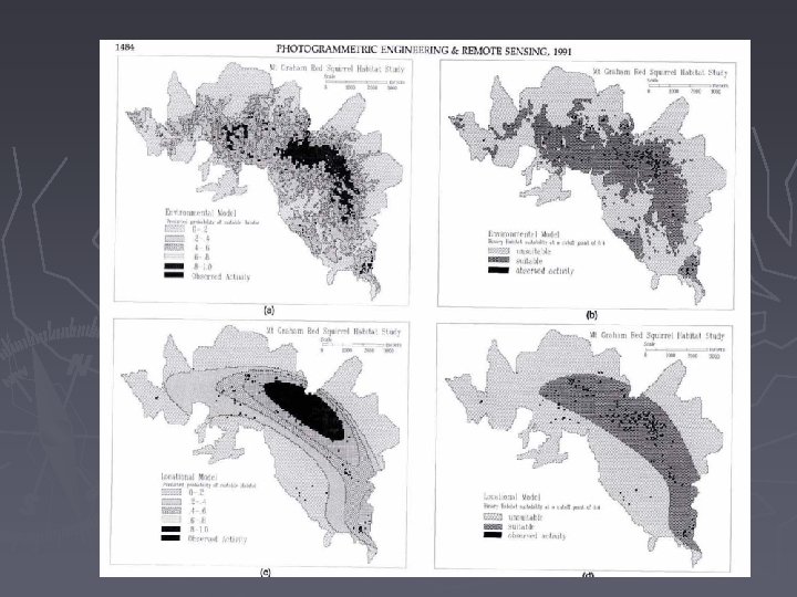
5. Model 1 - the Logistic Model Y = 0. 002 ele - 0. 228 slope + 0. 685 canopy(high) + 0. 443 canopy(medium) + 0. 481 canopy(low) + 0. 009 aspect(e-w) P (Y) = 1/[1 + exp (-Y)] P - The probability of red squirrel habitat

Accuracy Assessment Matrix for the 150 presence and 150 absence sites that are used to develop the logistic model Truth ► Error Modeled presence absence presence 123 27 absence 36 114 total accuracy 150 82% 150 76% 300 Overall accuracy = (123+114)/300 = 79%

Model Validation Matrix for the 50 presence and 50 absence sites that are put aside for model validation Truth ► Error Modeled presence absence total accuracy 74% presence 37 13 50 68% absence 16 34 50 100 71%

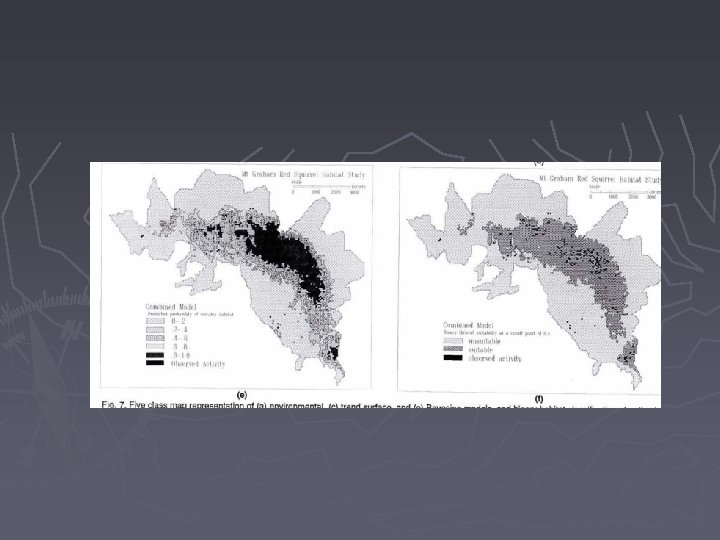
5. Model 2 - Trend Surface Analysis ► A dependent variable and two independent variables – x and y coordinates Linear (1 st order) : z = a 0 + a 1 x + a 2 y ► Quadratic (2 nd order): z = a 0 + a 1 x + a 2 y + a 3 x 2 + a 4 xy + a 5 y 2 ► Cubic etc. ► ► Least square method

Trends of one, two, and three independent variables for polynomial equations of the first, second, and third orders (after Harbaugh, 1964).

5. Trend Surface Analysis. . ► Assuming that the presence and absence depend on coordinates x and y ► A 4 th order polynomial multiple logistic regression model is used Dependent variable: presence and absence ► Independent variables: x and y ► Prediction accuracy: 57% ►

5. Model 3 - Bayesian Model A Bayesian model is used to combine the environmental model and the trend surface model ► to reach a predictive accuracy of 87% ►

6. Habitat Loss Estimate ► Total number of cells lost to the observatory: Overlay the predicted suitable cells and construction cells ► Density of red squirrel in each suitability class: number of presence in the class / acreage of the class ► Total habitat loss: S density * acreage per class