ENT 420 Biological System Modeling Systems of non

ENT 420 Biological System Modeling Systems of non linear ODEs Steady states and stability Lecturer Engr. Mohd Yusof bin Baharuddin MBiomed. Eng (Melbourne) BBiomed. Eng (Malaya)

ENT 420 Biological System Modeling Objective • Introduction to population models based on systems of nonlinear ordinary differential equations (ODEs) • Give names to new types of steady states

ENT 420 Biological System Modeling The real world may not be linear, but we try to pretend that it is • We can deal with the stability of systems of nonlinear ODEs by linearising them about critical points (e. g. steady states) • Once we have linearised our equations we can apply the same methods developed in for linear ODEs

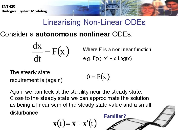
ENT 420 Biological System Modeling Linearising Non-Linear ODEs Consider a autonomous nonlinear ODEs: Where F is a nonlinear function e. g. F(x)=x 4 + x Log(x) The steady state requirement is (again) Again we can look at the stability near the steady state. Close to the steady state we can approximate the solution as being a linear sum of the steady state value and a small disturbance Familiar?

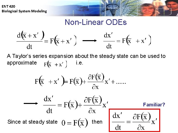
ENT 420 Biological System Modeling Non-Linear ODEs A Taylor’s series expansion about the steady state can be used to approximate i. e. Familiar? Since at steady state then

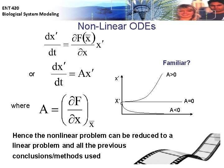
ENT 420 Biological System Modeling Non-Linear ODEs Familiar? or where x’ A>0 X’o A=0 A<0 Hence the nonlinear problem can be reduced to a linear problem and all the previous conclusions/methods used

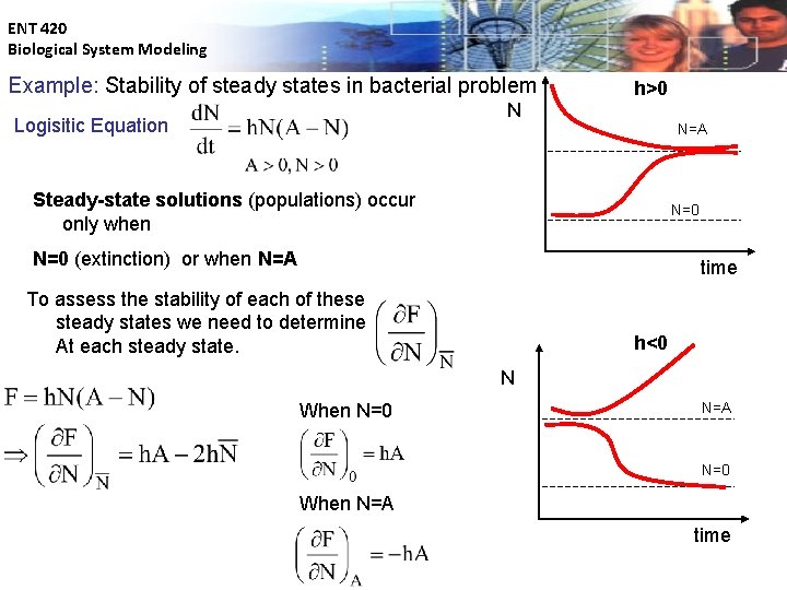
ENT 420 Biological System Modeling Example: Stability of steady states in bacterial problem h>0 N Logisitic Equation N=A Steady-state solutions (populations) occur only when N=0 (extinction) or when N=A time To assess the stability of each of these steady states we need to determine At each steady state. h<0 N When N=0 N=A N=0 When N=A time

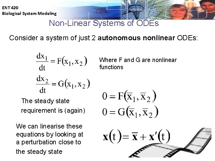
ENT 420 Biological System Modeling Non-Linear Systems of ODEs Consider a system of just 2 autonomous nonlinear ODEs: Where F and G are nonlinear functions The steady state requirement is (again) We can linearise these equations by looking at a perturbation close to the steady state

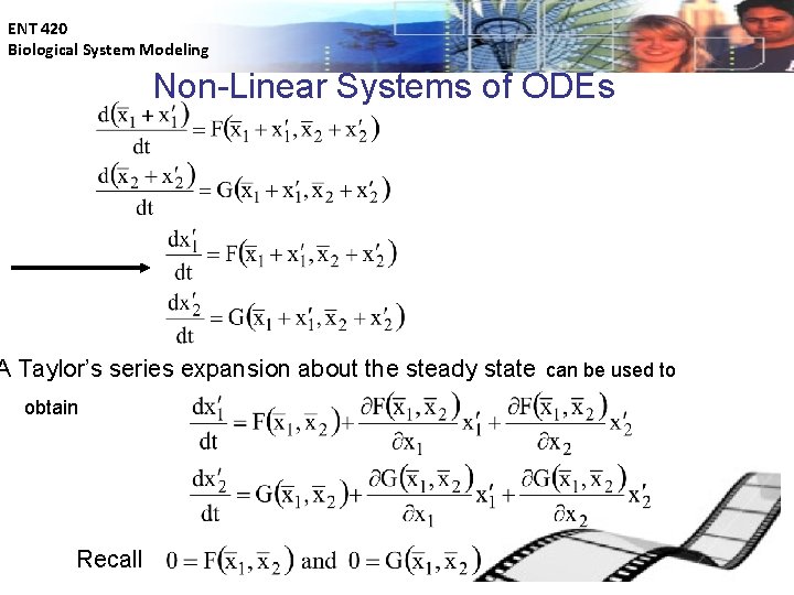
ENT 420 Biological System Modeling Non-Linear Systems of ODEs A Taylor’s series expansion about the steady state can be used to obtain Recall

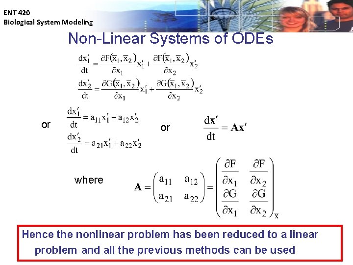
ENT 420 Biological System Modeling Non-Linear Systems of ODEs or or where Hence the nonlinear problem has been reduced to a linear problem and all the previous methods can be used

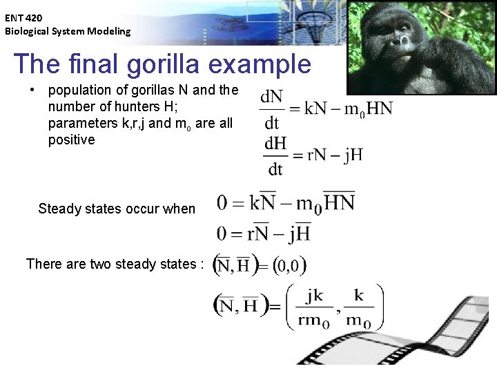
ENT 420 Biological System Modeling The final gorilla example • population of gorillas N and the number of hunters H; parameters k, r, j and mo are all positive Steady states occur when There are two steady states :

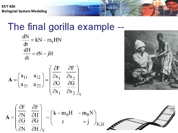
ENT 420 Biological System Modeling The final gorilla example --

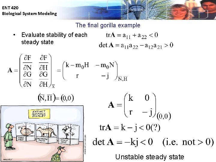
ENT 420 Biological System Modeling The final gorilla example • Evaluate stability of each steady state Unstable steady state

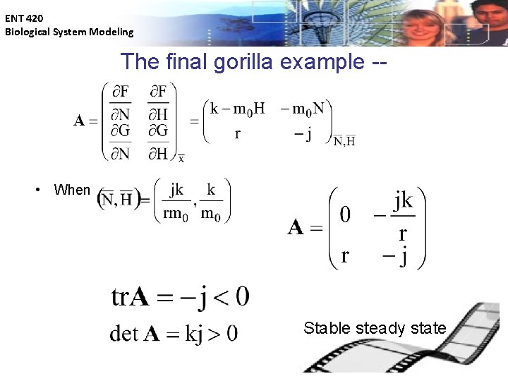
ENT 420 Biological System Modeling The final gorilla example -- • When Stable steady state

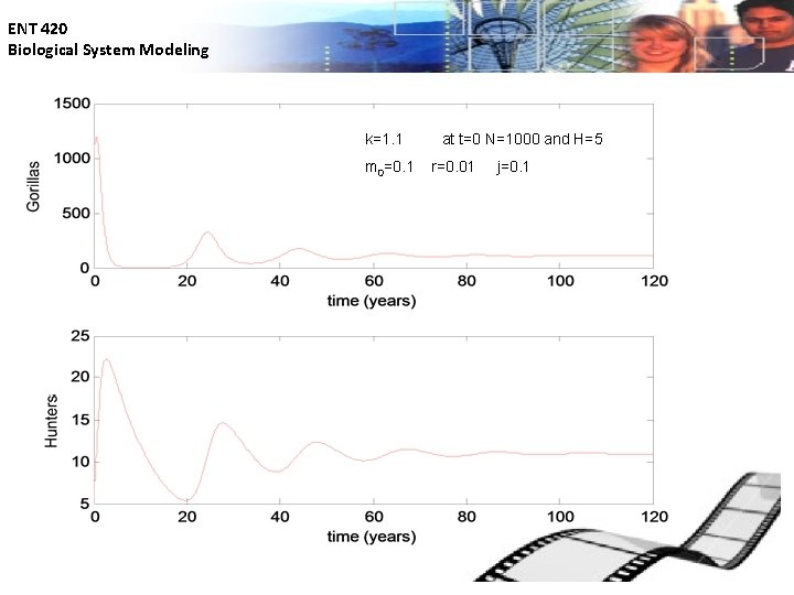
ENT 420 Biological System Modeling k=1. 1 m 0=0. 1 at t=0 N=1000 and H=5 r=0. 01 j=0. 1

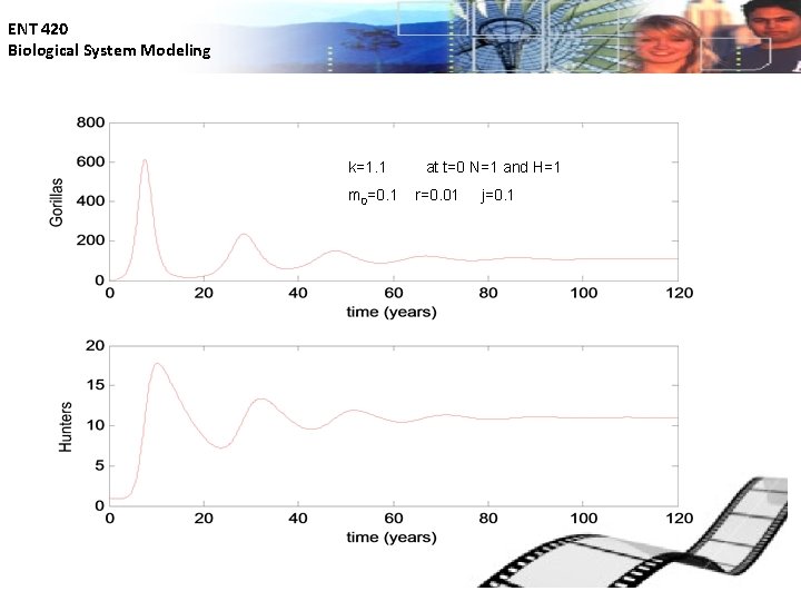
ENT 420 Biological System Modeling k=1. 1 m 0=0. 1 at t=0 N=1 and H=1 r=0. 01 j=0. 1

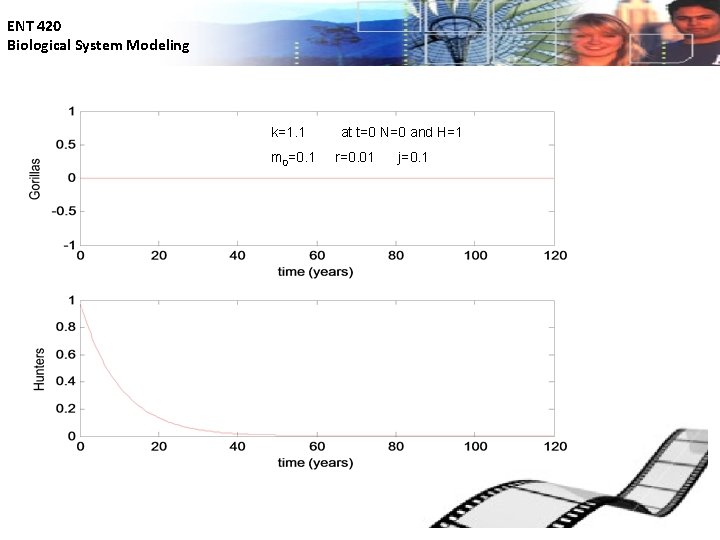
ENT 420 Biological System Modeling k=1. 1 m 0=0. 1 at t=0 N=0 and H=1 r=0. 01 j=0. 1

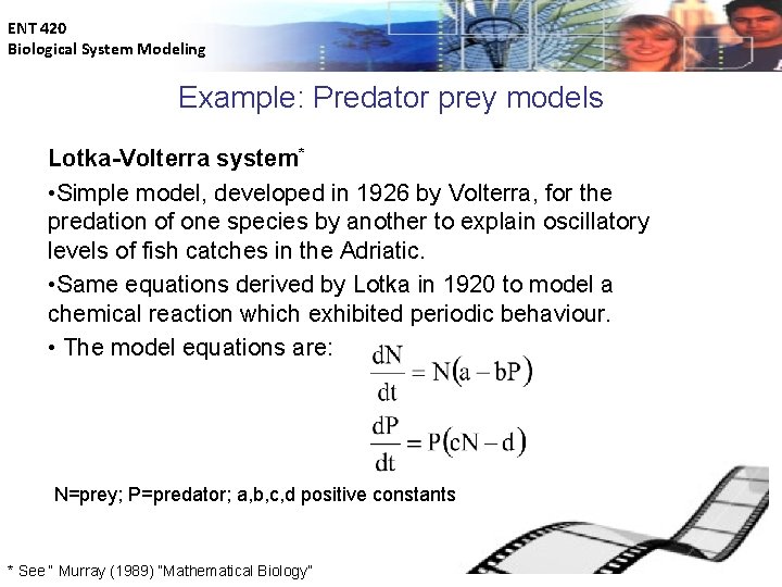
ENT 420 Biological System Modeling Example: Predator prey models Lotka-Volterra system* • Simple model, developed in 1926 by Volterra, for the predation of one species by another to explain oscillatory levels of fish catches in the Adriatic. • Same equations derived by Lotka in 1920 to model a chemical reaction which exhibited periodic behaviour. • The model equations are: N=prey; P=predator; a, b, c, d positive constants * See “ Murray (1989) “Mathematical Biology”

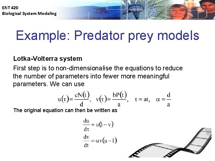
ENT 420 Biological System Modeling Example: Predator prey models Lotka-Volterra system First step is to non-dimensionalise the equations to reduce the number of parameters into fewer more meaningful parameters. We can use The original equation can then be written as

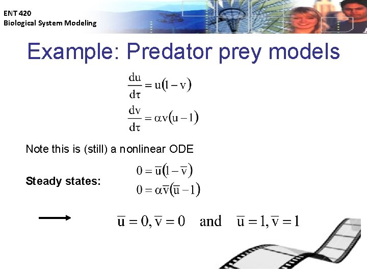
ENT 420 Biological System Modeling Example: Predator prey models Note this is (still) a nonlinear ODE Steady states:

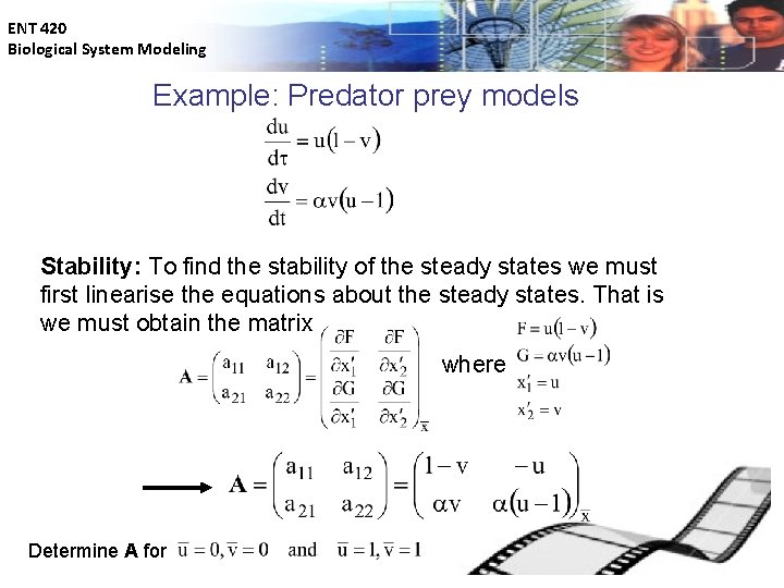
ENT 420 Biological System Modeling Example: Predator prey models Stability: To find the stability of the steady states we must first linearise the equations about the steady states. That is we must obtain the matrix where Determine A for

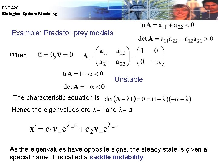
ENT 420 Biological System Modeling Example: Predator prey models When Unstable The characteristic equation is Hence the eigenvalues are =1 and =-α As the eigenvalues have opposite signs, the steady state is given a special name. It is called a saddle instability.

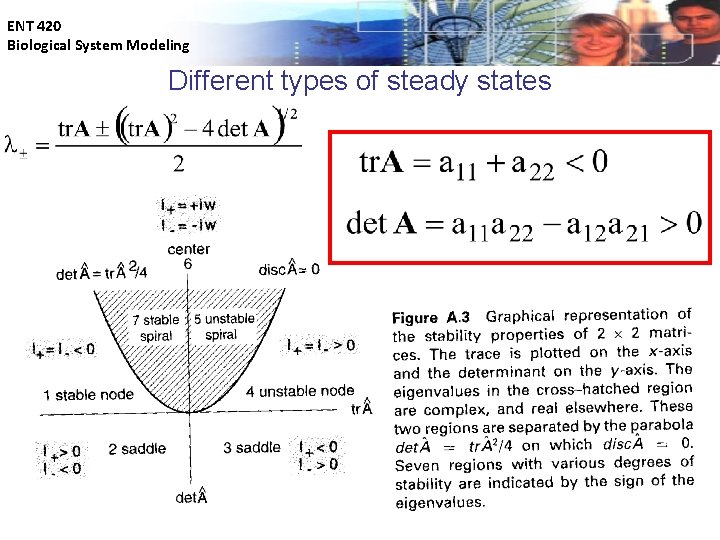
ENT 420 Biological System Modeling Different types of steady states

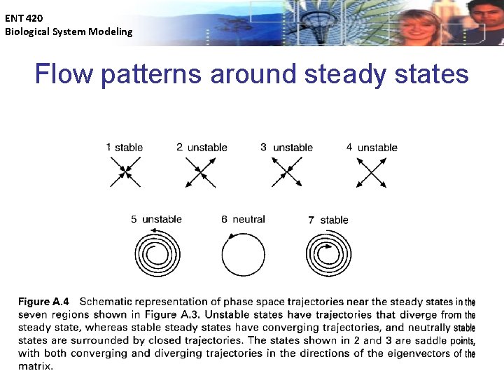
ENT 420 Biological System Modeling Flow patterns around steady states

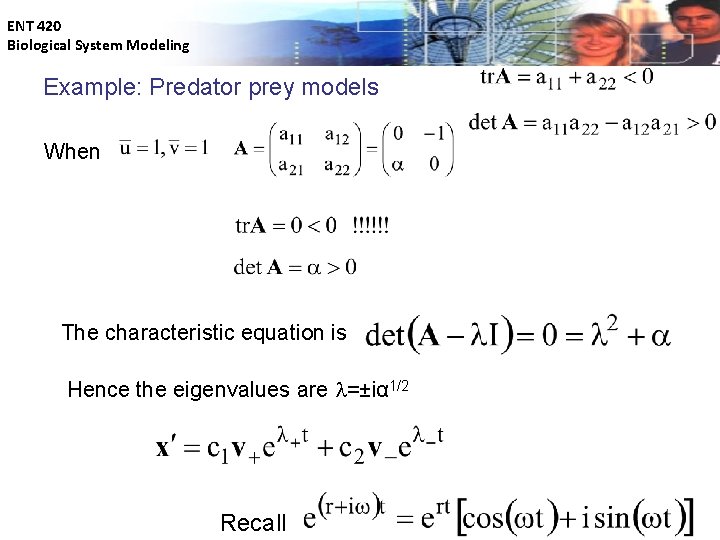
ENT 420 Biological System Modeling Example: Predator prey models When The characteristic equation is Hence the eigenvalues are =±iα 1/2 Recall

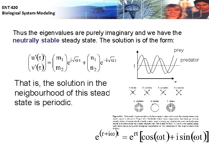
ENT 420 Biological System Modeling Thus the eigenvalues are purely imaginary and we have the neutrally stable steady state. The solution is of the form: prey predator 1 That is, the solution in the neigbourhood of this steady state is periodic.

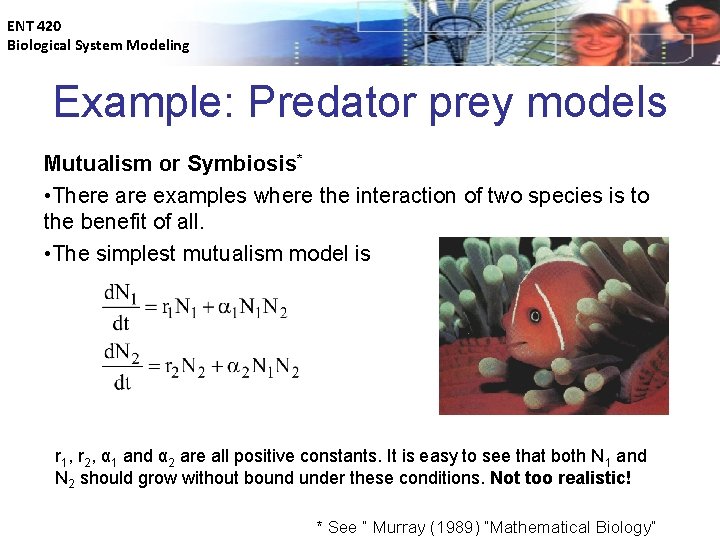
ENT 420 Biological System Modeling Example: Predator prey models Mutualism or Symbiosis* • There are examples where the interaction of two species is to the benefit of all. • The simplest mutualism model is r 1, r 2, α 1 and α 2 are all positive constants. It is easy to see that both N 1 and N 2 should grow without bound under these conditions. Not too realistic! * See “ Murray (1989) “Mathematical Biology”

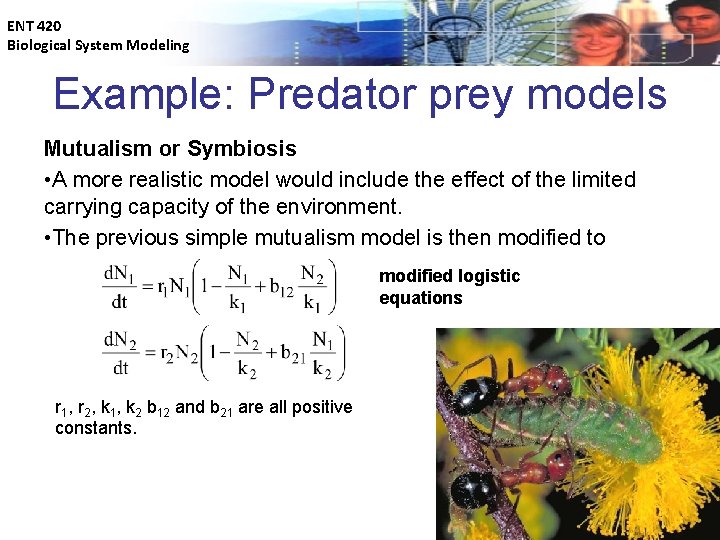
ENT 420 Biological System Modeling Example: Predator prey models Mutualism or Symbiosis • A more realistic model would include the effect of the limited carrying capacity of the environment. • The previous simple mutualism model is then modified to modified logistic equations r 1, r 2, k 1, k 2 b 12 and b 21 are all positive constants.

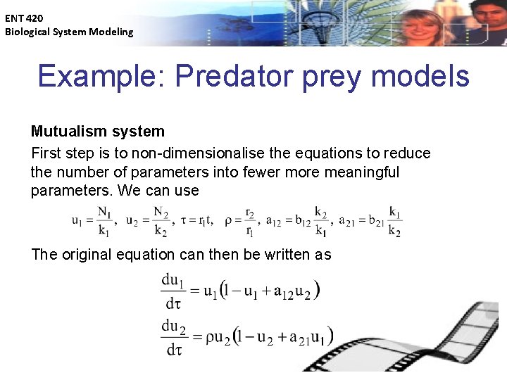
ENT 420 Biological System Modeling Example: Predator prey models Mutualism system First step is to non-dimensionalise the equations to reduce the number of parameters into fewer more meaningful parameters. We can use The original equation can then be written as

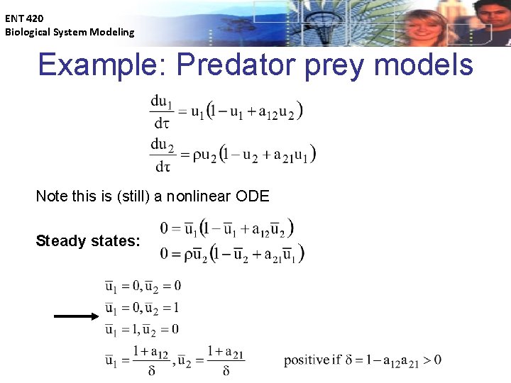
ENT 420 Biological System Modeling Example: Predator prey models Note this is (still) a nonlinear ODE Steady states:

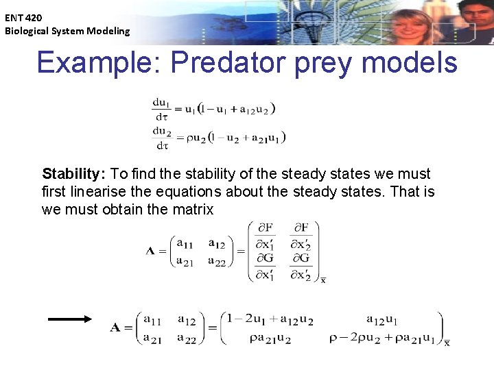
ENT 420 Biological System Modeling Example: Predator prey models Stability: To find the stability of the steady states we must first linearise the equations about the steady states. That is we must obtain the matrix

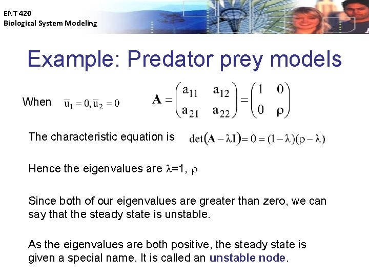
ENT 420 Biological System Modeling Example: Predator prey models When The characteristic equation is Hence the eigenvalues are =1, Since both of our eigenvalues are greater than zero, we can say that the steady state is unstable. As the eigenvalues are both positive, the steady state is given a special name. It is called an unstable node.

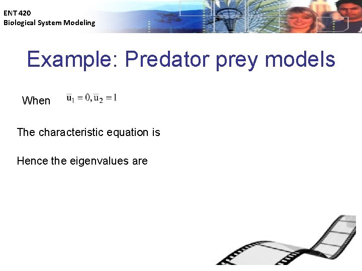
ENT 420 Biological System Modeling Example: Predator prey models When The characteristic equation is Hence the eigenvalues are

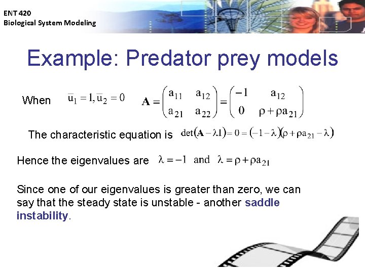
ENT 420 Biological System Modeling Example: Predator prey models When The characteristic equation is Hence the eigenvalues are Since one of our eigenvalues is greater than zero, we can say that the steady state is unstable - another saddle instability.

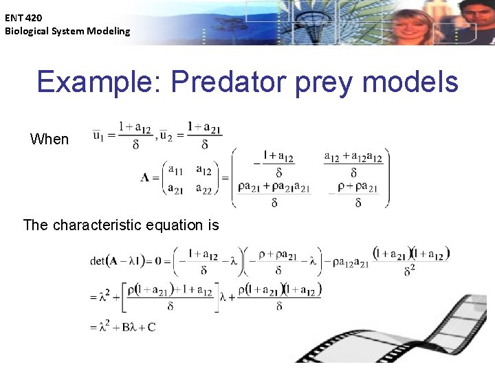
ENT 420 Biological System Modeling Example: Predator prey models When The characteristic equation is

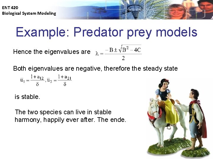
ENT 420 Biological System Modeling Example: Predator prey models Hence the eigenvalues are Both eigenvalues are negative, therefore the steady state is stable. The two species can live in stable harmony, happily ever after. The ende.

ENT 420 Biological System Modeling Example: Cancer modelling • • • Cancer development is regulated on many levels. On the subcellular level, mutations in a normal cell can result in a cancer cell phenotype. There are various mechanisms (systems) that the body (cell) uses to restrict these mutations. On a higher level, even a cancer cell phenotype that is capable of proliferating may not be able to form a tumour beyond a very small size. This is due to the body’s defences which try to prevent the growth and pathogenicity (ability to produce disease) of selfish transformed cells once they have been generated. The microenvironment in which the cancer cell emerges is thought to play a pivotal role in determining whether or not a cancer will succeed at growing to larger sizes. Blood supply is critical to this process, providing the necessary oxygen and nutrients to the cancer cell. Cancer cells must be able to induce the generation of new blood supply – a process called angiogenesis.

ENT 420 Biological System Modeling Angiogenesis http: //www. gene. com/gene/research/images/angiogenesis. jp

ENT 420 Biological System Modeling Cancer modelling • The ability of cancer cells to induce angiogenesis depends on a balance between angiogenesis promoters and angiogenesis inhibitors in the cancer cells microenvironment. • Examples of inhibitors are: thrombospondin, tumstatin, canstatin, endostatin, angiostatin and interferons • Examples of promoters are growth factors such as FGF, VEGF, IL-8 and PDGF. • Normal tissues mainly produce inhibitors – so do most cancers. • Angiogenic cancer cells have mutations which allow the balance between inhibitors and promoters to be pushed in favour of the promoters. This is done by either activating the production of promoters or inhibiting the production of inhibitors. • Chemotherapy now includes drugs which inhibits angiogenesis

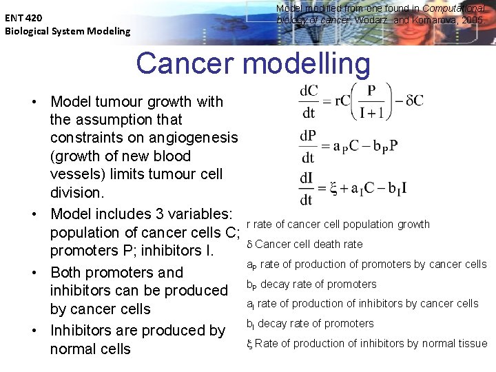
Model modified from one found in Computational biology of cancer, Wodarz and Komarova, 2005. ENT 420 Biological System Modeling Cancer modelling • Model tumour growth with the assumption that constraints on angiogenesis (growth of new blood vessels) limits tumour cell division. • Model includes 3 variables: population of cancer cells C; promoters P; inhibitors I. • Both promoters and inhibitors can be produced by cancer cells • Inhibitors are produced by normal cells r rate of cancer cell population growth Cancer cell death rate a. P rate of production of promoters by cancer cells b. P decay rate of promoters a. I rate of production of inhibitors by cancer cells b. I decay rate of promoters Rate of production of inhibitors by normal tissue

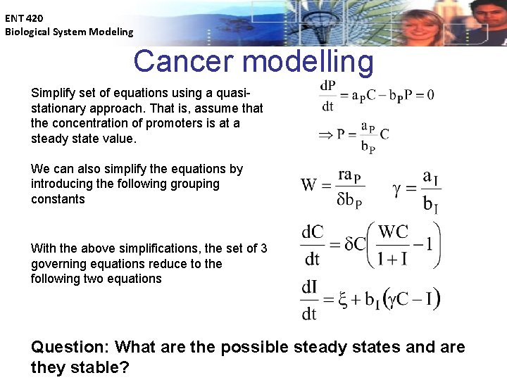
ENT 420 Biological System Modeling Cancer modelling Simplify set of equations using a quasistationary approach. That is, assume that the concentration of promoters is at a steady state value. We can also simplify the equations by introducing the following grouping constants With the above simplifications, the set of 3 governing equations reduce to the following two equations Question: What are the possible steady states and are they stable?

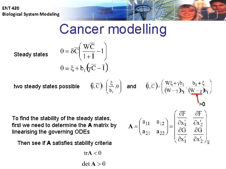
ENT 420 Biological System Modeling Cancer modelling Steady states two steady states possible and >0 To find the stability of the steady states, first we need to determine the A matrix by linearising the governing ODEs Then see if A satisfies stability criteria

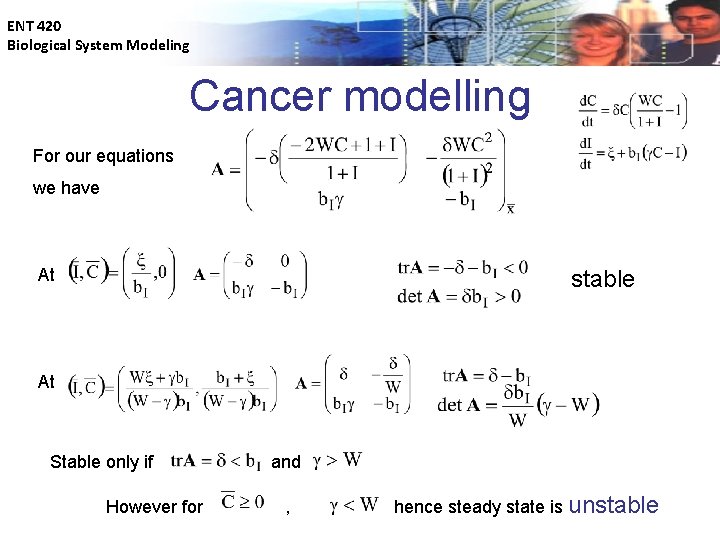
ENT 420 Biological System Modeling Cancer modelling For our equations we have At stable At Stable only if However for and , hence steady state is unstable

ENT 420 Biological System Modeling Summary • Introduction to steady states and stability analysis of systems of nonlinear ODEs • Examples of predator-prey models • Example of angiogenesis dependent cancer growth models • Introduction to names given to types of steady states

ENT 420 Biological System Modeling Sometimes seeing things need a skills to be polished…. ~Yusof~