EnsembleBased Data Assimilation Model PostProcessing and Regional NWP

Ensemble-Based Data Assimilation, Model Post-Processing, and Regional NWP Initial Results of the University of Washington CSTAR Project Greg Hakim & Cliff Mass University of Washington 29 April 2005

UW CSTAR • Leverages large regional prediction infrastructure. • Built on long-term cooperation between UW and Northwest NWS offices and Western Region. • Broad goal: develop and test new prediction approaches applicable not only to the western U. S. but the entire country.

UW CSTAR Specific Goals • Develop an En. KF data assimilation system. • Evaluate high-resolution ensemble forecasts. • Develop post-processing tools for grid-based model bias removal for use in IFPS. • Evaluate high-resolution prediction over the NW, including testing of WRF.

UW CSTAR Specific Goals • Maintain & expand the Northwest regional data collection system. – new QC and mesoscale verification tools. • Real-time coupled atmos-hydro forecasting – including forcing by atmospheric ensembles. • Experimental En. KF-based Analysis of Record (AOR).
 • Ryan Torn thesis")
UW Data Assimilation Research • Ensemble Kalman Filter (En. KF) • Ryan Torn thesis research. • Sebastien Dirren.

En. KF Basic Idea ��� ��� Analyses observation assimilation ��� model runs ��� Forecasts Analyses

Gaussian Update analysis = background + weighted observations innovation: new obs information Kalman gain matrix
 Algorithm (1) Ensemble forecast provides background estimate")
Summary of Ensemble Kalman Filter (En. KF) Algorithm (1) Ensemble forecast provides background estimate & statistics (B) for new analyses. (2) Ensemble analysis with new observations. (3) Ensemble forecast to arbitrary future time.

En. KF Pros & Cons Pros: • Flow-dependent background-error covariance. • Scale-independent approach. –mesoscale, complex topography, cloud fields. Cons: • Rank deficient ensembles. –covariance “inflation” & “localization” often used. • no help for near-field cross-variable covariance. • Calculation scales with number of observations.

When is the En. KF Most Useful? • Sparse observations. • Mesoscale circulations. • Complex topography. Little advantage over 3 DVAR for: • dense observations. • synoptic/planetary-scale analyses. • conventional balances apply.

Ensemble Covariance Examples

Temperature-Temperature Covariance 3 D-VAR covariance ensemble covariance

Temperature-Wind Covariance 3 D-VAR covariance ensemble covariance
")
Mesoscale Example: cov(|V|, qrain)

Limited-area En. KFs • Most En. KF development for global models. • Limited-area En. KFs require ensemble BCs. • Several options available (Torn et al. 2005). • Here we use random draws from N(0, B). • B = WRF 3 DVAR covariance model. • Red noise process in time. • Perts centered on GFS 12 - hour forecast. • Affects ~100 km wide region near lat. bndrs.

UW Real-time En. KF • 90 member ensemble for analyses & forecasts. • 45 km grid over E. Pac & W. NOAM. • 6 -hour assimilation cycle. • Observations assimilated (~5000 -8000 per time): • Radiosondes. • ACARS. • Surface: ASOS, ships, buoys. • Cloud-track winds. • Availability ~t+3 hours. • 24 -h forecasts: 00 & 12 UTC. • Available ~t+5. 5 hours.

U. Washington Real-time En. KF http: //www. atmos. washington. edu/~enkf

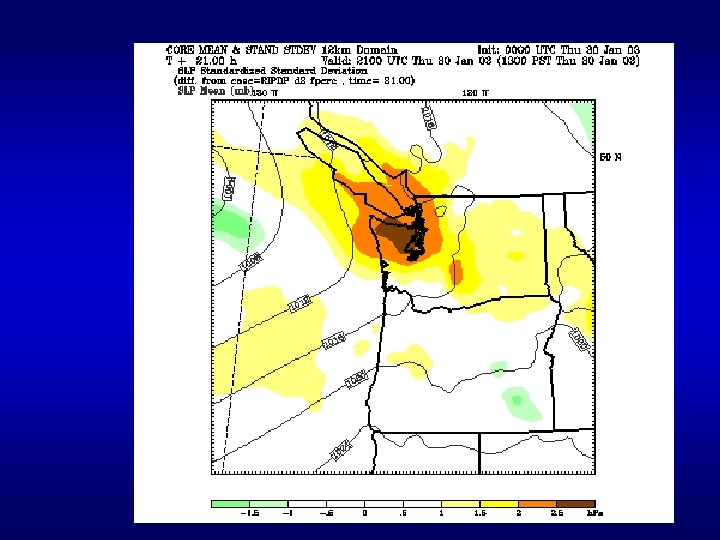
Probabilistic Analyses sea-level pressure 500 h. Pa height Large uncertainty associated with shortwave approaching in NW flow

Ensemble Forecasts Analysis 24 -hour forecast

Ensemble Forecasts Analysis 24 -hour forecast

Sfc P 24 h Forecast Sensitivity

Surface Pressure Verification Red = UW En. KF ensemble mean Green = UW En. KF ensemble members Blue = NCEP GFS

500 h. Pa Height Verification Red = UW En. KF ensemble mean Green = UW En. KF ensemble members Blue = NCEP GFS

Sensitivity Example analysis SLP 850 h. Pa temp.

SLP Climatological Sensitivity Sea-level pressure 500 h. Pa height

15 km Nested-Grid Experiment • Nested domain. • BCs from 45 km En. KF. • Assimilation every 3 hours over 48 h period.

Surface Winds

Radar Reflectivity

Reflectivity Analysis & Increment More precip over most of region; NW shift of primary band

Current & Future Plans • Nested grids at higher resolution. AOR • 15 km & 5 km. • More frequent updates. • every 3 -hours, then hourly. • also try “cheap” hourly updates. • Update key fields only; no propagation; available ~t+15 min. • Ensemble Kalman smoother. AOR • Use observations to update earlier analyses. • Satellite radiance assimilation.

Grid-Based Model Bias Removal: We All Need It! Model biases are a reality We need to get rid of them

Grid-Based Bias Removal • In the past, the NWS has attempted to remove these biases only at observation locations (MOS, Perfect Prog) • Removal of systemic model bias on forecast grids is needed: – All models have significant systematic biases – NWS and others want to distribute graphical forecasts on a grid (IFPS) – People and applications need accurate forecasts everywhere…not only at ASOS sites – Important post-processing step for ensembles

How does one do it? • One cannot simply calculate the biases at observation locations and then spread them around with standard interpolation schemes. • Why? – Because you don’t want to spread the non-systematic biases particular to specific stations to their surroundings. – Because nearby stations might be of different elevation and land use…so even the systematic biases might differ.

A Potential Solution: Observation-Based Grid Based Bias Removal • Based on the biases of nearby observation sites. • Base the bias removal on observation-site land-use category, elevation, and proximity. Land use and elevation are key parameters the control physical biases. • Make use of parameter values to insure only applies observation locations of similar regimes.

Spatial differences in bias
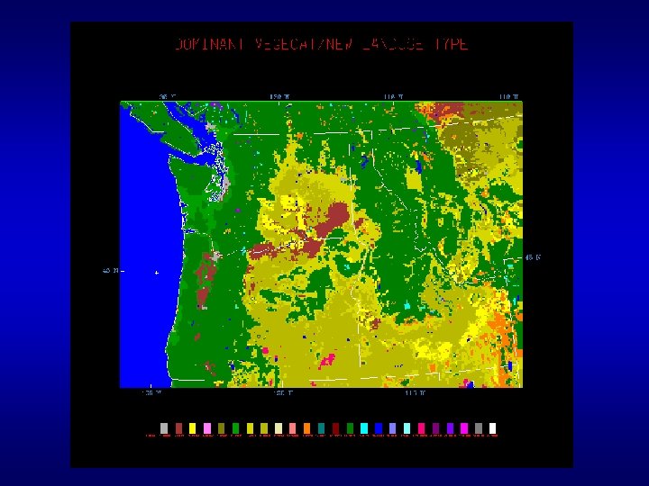

The Method § Calculate model biases at observation locations by interpolating model forecasts to observation sites. § Identify a land use, elevation, and lat-lon for each observation site. • Calculate biases at these stations hourly. Thus, one has a data-base of hourly biases. • For every forecast hour: At every forecast grid point search for nearby stations of similar land use and elevation and for which the previous forecast value is close to that forecast at the grid point in question. – E. g. , if the forecast temperature was 60, only use biases for nearby stations of similar land-use/elevation associated with forecasts of 55 -65. • Collect a sufficient number of these (using closest and most recent ones first) to average out local effects (roughly a half dozen). Average the biases for these sites and apply the bias correction to the forecast.

Grid-Base Bias Removal Why is this approach good? – Takes out diurnal bias – Takes in consideration land use (e. g. , land versus water and generally will only use stations from right side of mountains) – Does not spread representativeness error – Based on recent biases so adaptive for time of year and model changes – Only uses biases from similar regimes.

Raw 12 -h Forecast Bias-Corrected Forecast

Sal Lake City

Bozeman

Next Steps • We are now operationally running gridbased bias removal for Northwest MM 5 surface grids. • This month will begin shipping biascorrected grids to NWS for testing in IFPS. • Testing nationally?
 • How Good is WRF over")
WRF vs MM 5 (VS Eta and GFS) • How Good is WRF over the Western U. S. ? • How Does It Compare to MM 5, Eta, and GFS? • Does it Offer Substantial Benefits?
 • Until this year, the UW")
WRF vs MM 5 (VS Eta and GFS) • Until this year, the UW verification system was evaluating MM 5 (36 -12 -4 km), with NCEP Eta and GFS. • In January we began running WRF (ARWcore) at 36 -12 km (twice a day to 48 h) to provide a detailed comparison between WRF and the other models over the complex terrain and land-water contrasts of the Pacific Northwest. • Takes advantage of the extensive verification system already in place.

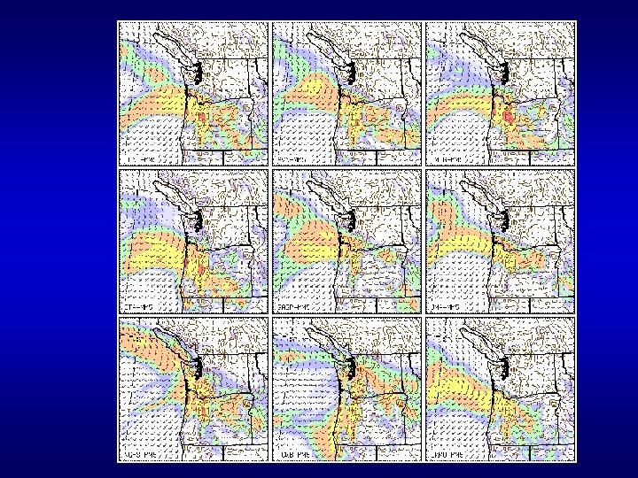
MM 5 1 K Winds WRF
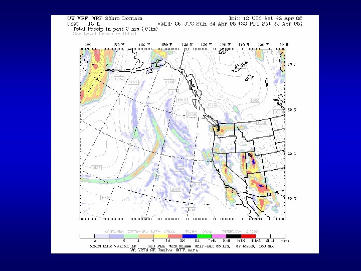
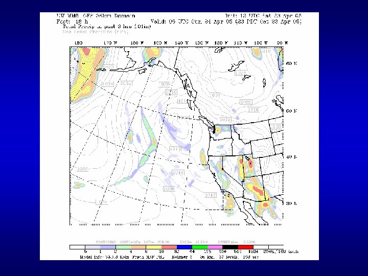

First Subjective Impressions • Low-level wind fields in terrain very similar. • This is also true of thermal fields. • WRF shows more structure in precipitation and tends to be more aggressive (although there are differences in microphysics schemes).
 to")
Next Steps • Add WRF ARW to objective verification system (now in progress) to provide real numbers regarding performance. • Add WRF NMM run when available. • Transition from MM 5 to WRF (best core) for regional NWP later this year if no negative impacts.

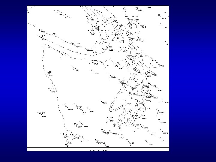
Regional Data Acquisition and Quality Control • The UW is now gathering data from roughly twodozen regional networks for both research and operations. • The UW network of networks (a. k. a Northwest Net) is distributed to the NWS and Mesowest. • With a heterogeneous observing network--made up of many networks-- a capable quality control system is required. • The Northwest challenge… develop a QC system viable in complex terrain and land/contrasts. This is not Kansas or Oklahoma!

Northwest. Net

20 April 2005 2200 UTC

UW QC Checks • Range Check A simple gross error check to make sure the observation is within a reasonable range. • Step Check This test looks for "spikes" in an station's time series for a given variable. Successive observations are compared and if the delta between them is above a set threhold, the value is flagged. • Persistence Check This test looks at the standard deviation of 24 hours of data for each station and variable. If the standard deviation is below a set minimum allowed value, all values in the 24 hour period are flagged at the "warning" level, depending on set thresholds.

QC Tests Spatial Check • This test compares each observation to those of surrounding stations of similar elevation. Looks within 100 -km for first try. Once it finds 5 stations, it checks if any of the stations has a similar parameter value (within some threshold), if not rejects the observation. If not 5, stations, looks farther.

Spatial QC in/near Terrain Easy Reject Accept

Network Statistics Available in Real-Time

Regional Verification • Critical for evaluating MM 5 and WRF • Most based on interpolating model output to observation locations.

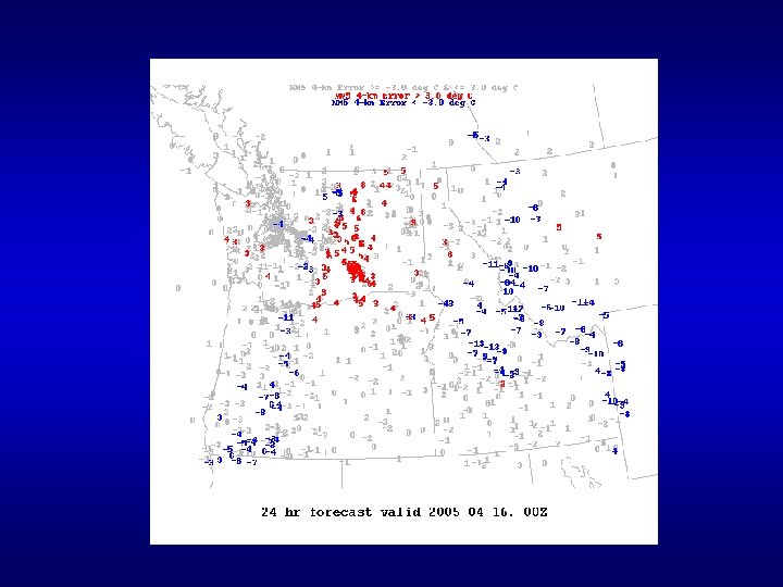
2 -m temperature

ACARS Verification

Soil Moisture Verification
, 17 members, is based")
Mesoscale Ensembles • The UW mesoscale ensemble system (3612 km), 17 members, is based on using initialization and BC from different analyses/forecasts of major NWP centers. Perhaps the highest resolution operational ensemble system in U. S. • Essentially a downscaling of a poor man ensemble from major operational centers. The idea is that such an ensemble would be a high bar to surpass– since its parent models are different (physics, numerics), observations used are different, and data assimilation approaches vary.
 Objective Analysis Abbreviation/Model/Source Type")
Current International Multi-Analysis Collection Resolution (~ @ 45 N ) Objective Analysis Abbreviation/Model/Source Type gfs, Global Forecast System, Spectral T 254 / L 64 ~55 km 1. 0 / L 14 ~80 km SSI 3 D Var Finite Diff. 0. 9 / L 28 ~70 km 1. 25 / L 11 ~100 km 3 D Var Finite Diff. 12 km / L 60 90 km / L 37 SSI 3 D Var Spectral T 239 / L 29 ~60 km 1. 0 / L 11 ~80 km 3 D Var Spectral T 106 / L 21 ~135 km 1. 25 / L 13 ~100 km OI Spectral T 239 / L 30 Fleet Numerical Meteorological & Oceanographic Cntr. ~60 km 1. 0 / L 14 ~80 km OI tcwb, Global Forecast System, 1. 0 / L 11 ~80 km OI National Centers for Environmental Prediction cmcg, Global Environmental Multi-scale (GEM), Canadian Meteorological Centre eta, Eta limited-area mesoscale model, National Centers for Environmental Prediction gasp, Global Analysi. S and Prediction model, Australian Bureau of Meteorology jma, Global Spectral Model (GSM), Japan Meteorological Agency Computational ngps, Navy Operational Global Atmos. Pred. System, Taiwan Central Weather Bureau ukmo, Unified Model, United Kingdom Meteorological Office Spectral T 79 / L 18 ~180 km Finite Diff. Distributed 5/6 5/9 /L 30 same / L 12 ~60 km 3 D Var

UW Ensemble • Recently, has been upgraded: twice a day and much earlier delivery for NWS use. • Considerable research on the applications of such ensembles for predicting forecast skill (Eric Grimit thesis) and ability of such ensembles to provide useful probabilistic guidance (Tony Eckel thesis)

Ensemble domain

What is the UWME? 2 Mesoscale Ensemble systems – Core : 8 members, 00 and 12 Z • Each uses different synoptic scale initial and boundary conditions • All use same physics – Physics : 8 members, 00 Z only • Each uses different synoptic scale initial and boundary conditions • Each uses different physics • Each uses different SST perturbations • Each uses different land surface characteristic perturbations – Centroid, 00 and 12 Z • Average of 8 core members used for initial and boundary conditions

UW Ensemble Web Page

48 h Probabilistic Forecast Of 1 inch In 12 h:

Verification Rank Histograms Bias Correction Is Very Important
 Z 500 VOP *UWME+ 5. 0 % 4.")
Comparison of 36 -h VRHs (a) Z 500 VOP *UWME+ 5. 0 % 4. 2 % *UWME+ 9. 0 % 6. 7 % *UWME+ 25. 6 % 13. 3 % *UWME+ 43. 7 % 21. 0 % (b) MSLP Synoptic Variable ( Errors Depend on Analysis Uncertainty ) (c) WS 10 Surface/Mesoscale Variable ( Errors Depend on Model Uncertainty ) (d) T 2

Now comparing the UW ensemble against the NCEP breeding-based mesoscale ensemble, and the UW En. KF ensemble system.

NCEP SREF vs UW Ensemble Bias Corrected Forecast Hour 39 h NCEP, 48 h UW, 20 -km RUC Verification

Ensemble Future • Major effort going into developing effective post-processing (e. g. , BMA…Bayesian Model Averaging) • Will develop better graphics and front end for use by forecasters. • Will be used to drive UW distributed hydrological prediction system. . . which is used by the NWS.

BMA PDF at a point For 48 -h 2 -m Temperature forecast

The End

NWS Forecaster vs MOS Verification
. • 30 stations,")
Data • July 1 2003 – Jan 1 2004 (6 months). • 30 stations, all at major WFO sites. • Maximum and minimum temperature, and POP.
 for the seven forecast types for all stations, all time periods,")
MAE ( F) for the seven forecast types for all stations, all time periods, 1 August 2003 – 1 August 2004.

MAE for each forecast type during periods of large temperature change (10 F over 24 -hr), 1 August 2003 – 1 August 2004. Includes data for all stations.
 from daily")
MAE for each forecast type during periods of large departure (20 F) from daily climatological values, 1 August 2003 – 1 August 2004.

Brier Scores for the seven forecasts for all stations for the entire study period.

MOS has periods of considerable bias…some of which humans can correct
- Slides: 85