Ensemble methods The slides are closely adapted from

Ensemble methods The slides are closely adapted from Subhransu Maji’s slides

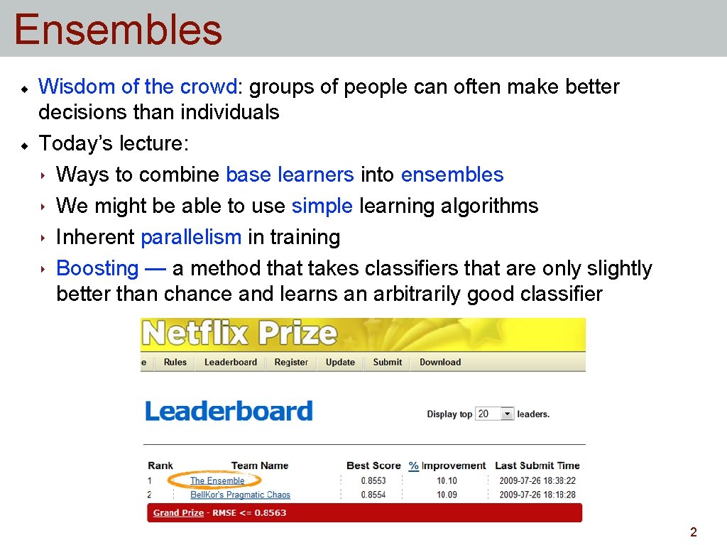
Ensembles Wisdom of the crowd: groups of people can often make better decisions than individuals Today’s lecture: ‣ Ways to combine base learners into ensembles ‣ We might be able to use simple learning algorithms ‣ Inherent parallelism in training ‣ Boosting — a method that takes classifiers that are only slightly better than chance and learns an arbitrarily good classifier 2

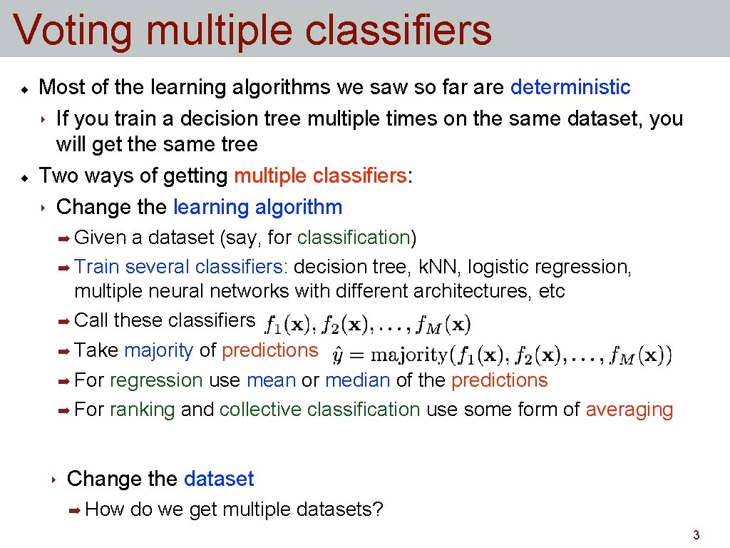
Voting multiple classifiers Most of the learning algorithms we saw so far are deterministic ‣ If you train a decision tree multiple times on the same dataset, you will get the same tree Two ways of getting multiple classifiers: ‣ Change the learning algorithm ➡ Given a dataset (say, for classification) ➡ Train several classifiers: decision tree, k. NN, logistic regression, multiple neural networks with different architectures, etc ➡ Call these classifiers ➡ Take majority of predictions ➡ For regression use mean or median of the predictions ➡ For ranking and collective classification use some form of averaging ‣ Change the dataset ➡ How do we get multiple datasets? 3

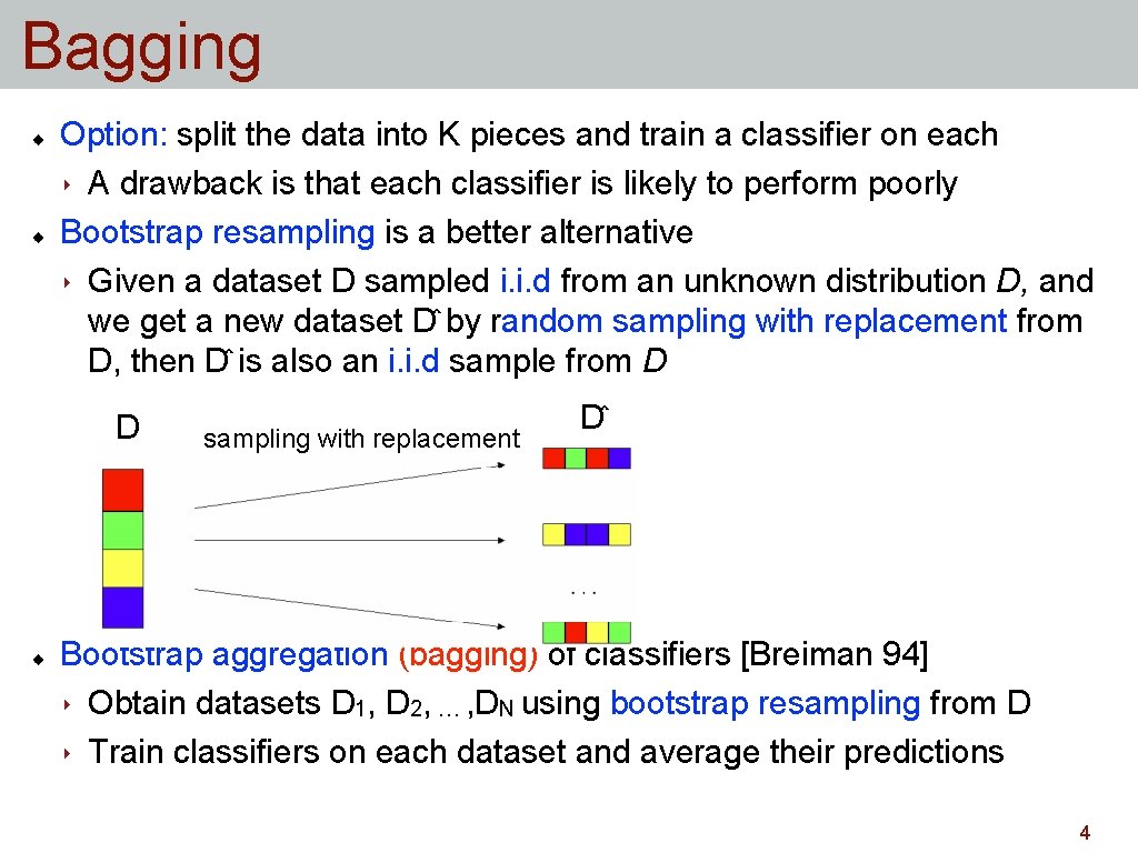
Bagging Option: split the data into K pieces and train a classifier on each ‣ A drawback is that each classifier is likely to perform poorly Bootstrap resampling is a better alternative ‣ Given a dataset D sampled i. i. d from an unknown distribution D, and we get a new dataset D by random sampling with replacement from D, then D is also an i. i. d sample from D D sampling with replacement D Bootstrap aggregation (bagging) of classifiers [Breiman 94] ‣ Obtain datasets D 1, D 2, … , DN using bootstrap resampling from D ‣ Train classifiers on each dataset and average their predictions 4

Why does averaging work? Averaging reduces the variance of estimators 50 samples Averaging is a form of regularization: each model can individually overfit but the average is able to overcome the overfitting 5

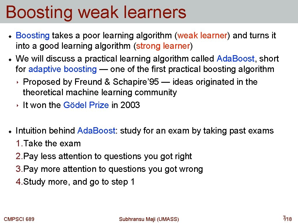
Boosting weak learners Boosting takes a poor learning algorithm (weak learner) and turns it into a good learning algorithm (strong learner) We will discuss a practical learning algorithm called Ada. Boost, short for adaptive boosting — one of the first practical boosting algorithm ‣ Proposed by Freund & Schapire’ 95 — ideas originated in theoretical machine learning community ‣ It won the Gödel Prize in 2003 Intuition behind Ada. Boost: study for an exam by taking past exams 1. Take the exam 2. Pay less attention to questions you got right 3. Pay more attention to questions you got wrong 4. Study more, and go to step 1 CMPSCI 689 Subhransu Maji (UMASS) 7/18

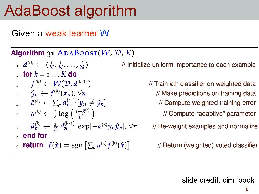
Ada. Boost algorithm Given a weak learner W slide credit: ciml book 8

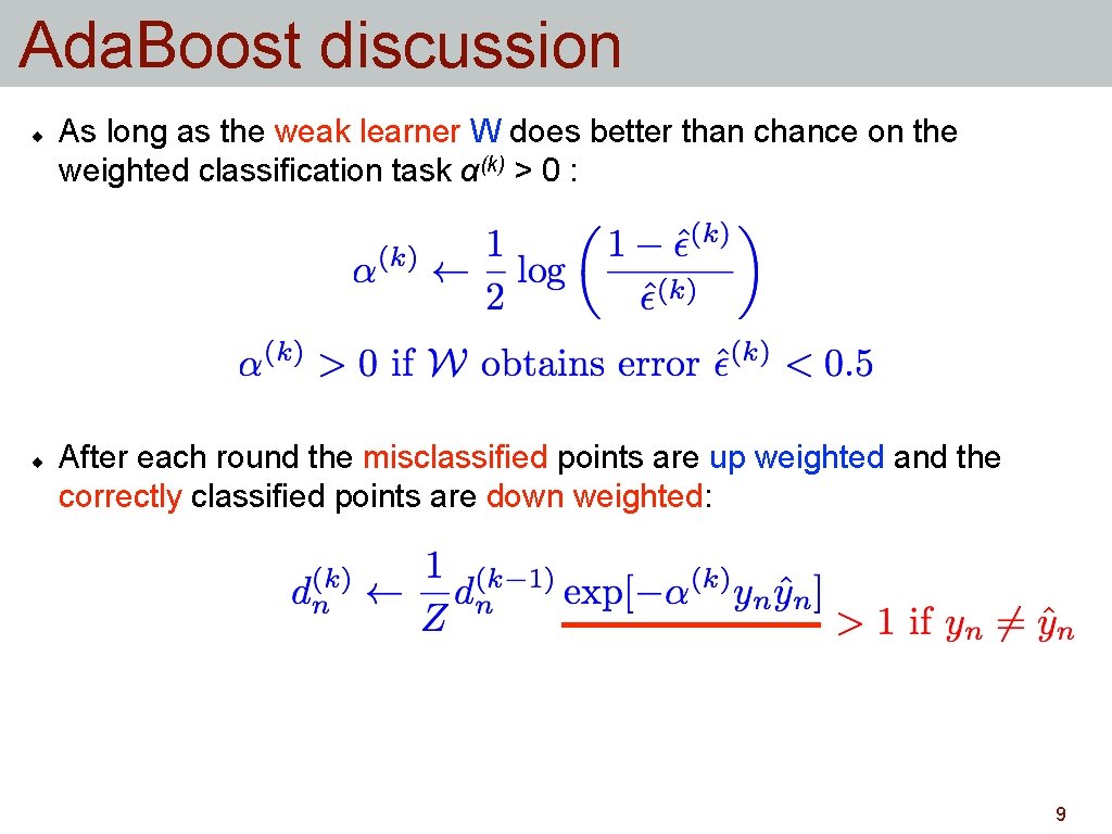
Ada. Boost discussion As long as the weak learner W does better than chance on the weighted classification task α(k) > 0 : After each round the misclassified points are up weighted and the correctly classified points are down weighted: 9

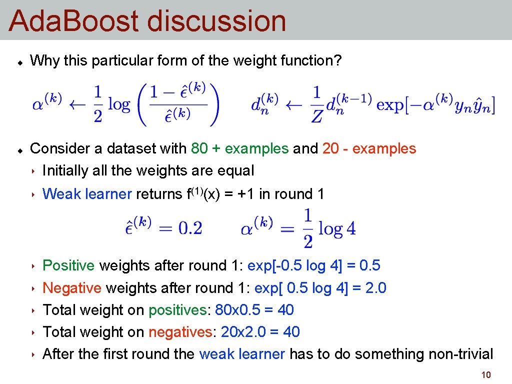
Ada. Boost discussion Why this particular form of the weight function? Consider a dataset with 80 + examples and 20 - examples ‣ Initially all the weights are equal ‣ Weak learner returns f(1)(x) = +1 in round 1 ‣ Positive weights after round 1: exp[-0. 5 log 4] = 0. 5 Negative weights after round 1: exp[ 0. 5 log 4] = 2. 0 Total weight on positives: 80 x 0. 5 = 40 Total weight on negatives: 20 x 2. 0 = 40 After the first round the weak learner has to do something non-trivial ‣ ‣ 10

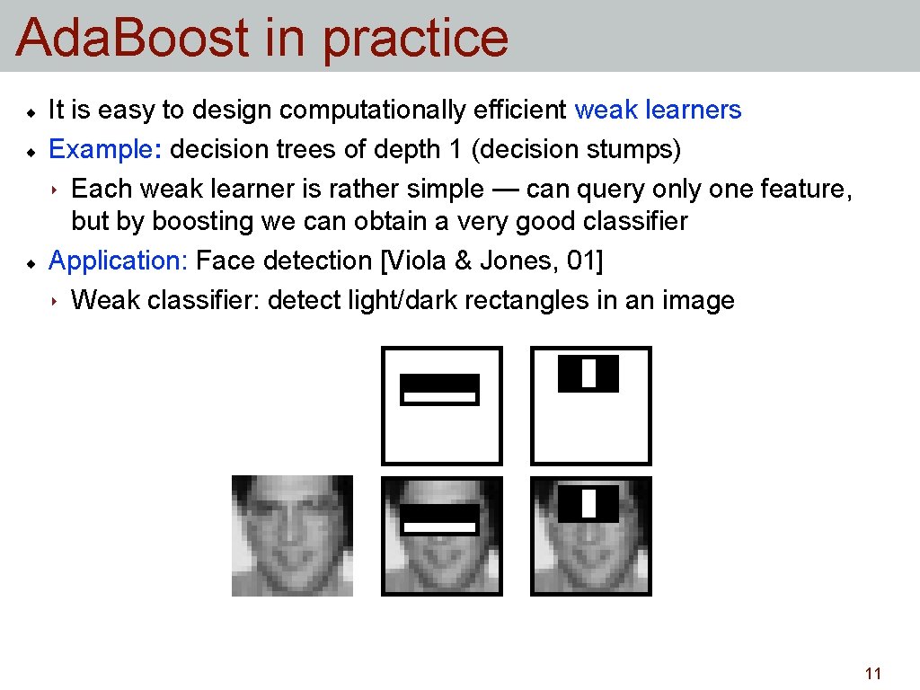
Ada. Boost in practice It is easy to design computationally efficient weak learners Example: decision trees of depth 1 (decision stumps) ‣ Each weak learner is rather simple — can query only one feature, but by boosting we can obtain a very good classifier Application: Face detection [Viola & Jones, 01] ‣ Weak classifier: detect light/dark rectangles in an image 11

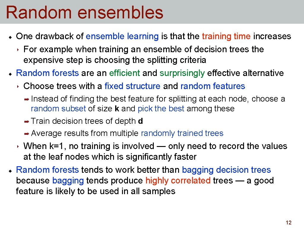
Random ensembles One drawback of ensemble learning is that the training time increases ‣ For example when training an ensemble of decision trees the expensive step is choosing the splitting criteria Random forests are an efficient and surprisingly effective alternative ‣ Choose trees with a fixed structure and random features ➡ Instead of finding the best feature for splitting at each node, choose a random subset of size k and pick the best among these ➡ Train decision trees of depth d ➡ Average results from multiple randomly trained trees When k=1, no training is involved — only need to record the values at the leaf nodes which is significantly faster Random forests tends to work better than bagging decision trees because bagging tends produce highly correlated trees — a good feature is likely to be used in all samples ‣ 12

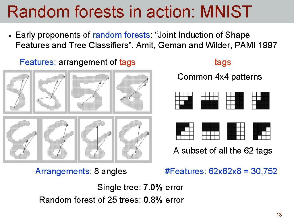
Random forests in action: MNIST Early proponents of random forests: “Joint Induction of Shape Features and Tree Classifiers”, Amit, Geman and Wilder, PAMI 1997 Features: arrangement of tags Common 4 x 4 patterns A subset of all the 62 tags Arrangements: 8 angles #Features: 62 x 8 = 30, 752 Single tree: 7. 0% error Random forest of 25 trees: 0. 8% error 13

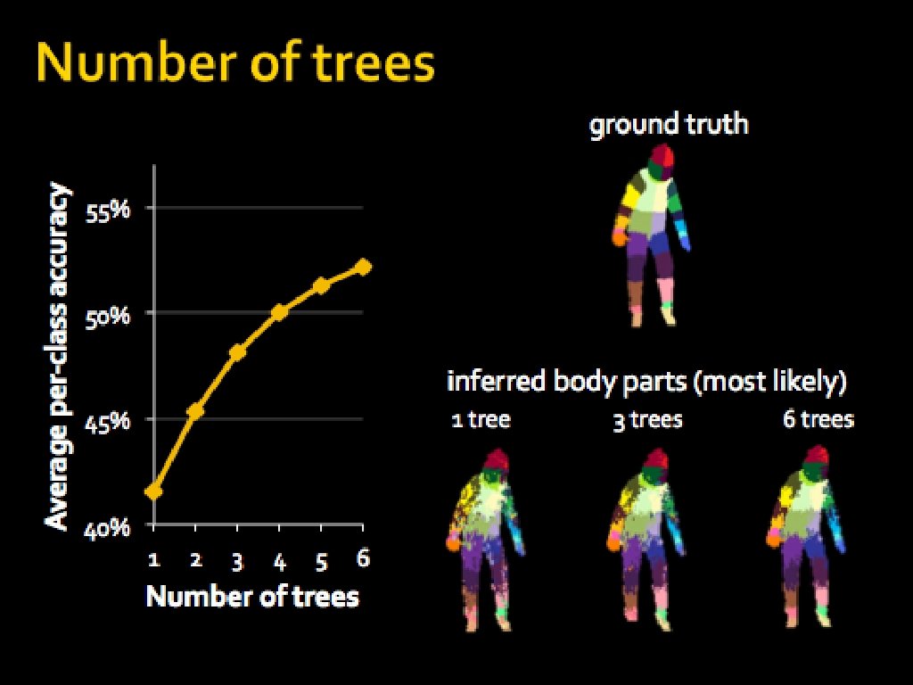
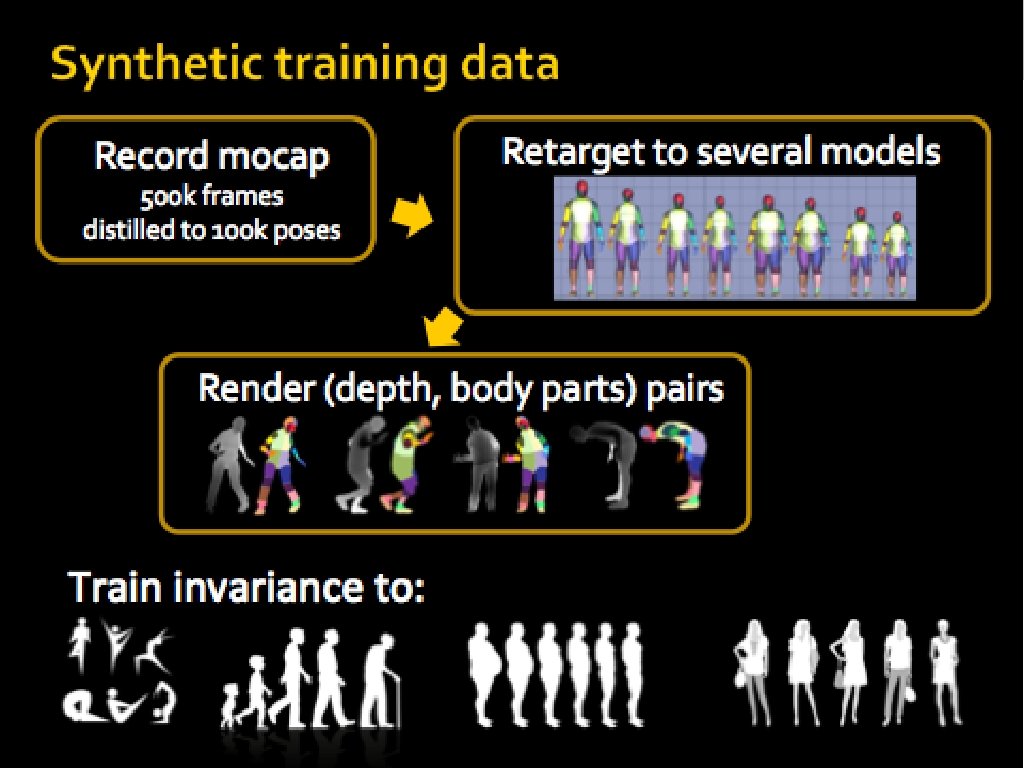
Random forests in action: Kinect pose Human pose estimation from depth in the Kinect sensor [Shotton et al. CVPR 11] Training: 3 trees, 20 deep, 300 k training images per tree, 2000 training example pixels per image, 2000 candidate features θ, and 50 candidate thresholds τ per feature (Takes about 1 day on a 1000 core cluster) 14

15

16

Summary Ensembles improve prediction by reducing the variance Two ways of creating ensembles ‣ Vary the learning algorithm ➡ Training algorithms: decision trees, k. NN, perceptron ➡ Hyperparameters: number of layers in a neural network ➡ Randomness in training: initialization, random subset of features ‣ Vary the training data ➡ Bagging: average predictions of classifiers trained on bootstrapped samples of the original training data Boosting combines weak learners to make a strong learner ‣ Reduces bias of the weak learners Ensembles of randomly trained decision trees are efficient and effective for many problems 17

Slides credit Slides are adapted from Subhransu Maji’s course Some of the slides are based on CIML book by Hal Daume III Bias-variance figures — https: //theclevermachine. wordpress. com/tag/estimator-variance/ Figures for random forest classifier on MNIST dataset — Amit, Geman and Wilder, PAMI 1997 — http: //www. cs. berkeley. edu/~malik/cs 294/amitgemanwilder 97. pdf Figures for Kinect pose — “Real-Time Human Pose Recognition in Parts from Single Depth Images”, J. Shotton, A. Fitzgibbon, M. Cook, T. Sharp, R. Moore, A. Kipman, A. Blake, CVPR 2011 18